(ADD INTRODUCTORY LANGUAGE ABOUT PROBLEM DEVELOPMENT) We will now consider two examples of bifurcation of equilibria in two dimensional Hamiltonian system; in particular, the Hamiltonian saddle-node and Hamiltonian pitchfork bifurcations.
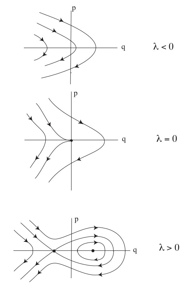
We consider the Hamiltonian:
H(q,p)=p22−λq+q33,(q,p)∈R2.where λ is considered to be a parameter that can be varied. From this Hamiltonian, we derive Hamilton's equations:
˙q=∂H∂p=p,˙p=−∂H∂q=λ−q2.The fixed points for (2) are:
(q,p)=(±√λ,0),from which it follows that there are no fixed points for λ<0, one fixed point for λ=0, and two fixed points for λ>0. This is the scenario for a saddle-node bifurcation.
Next we examine the stability of the fixed points. The Jacobian of (2) is given by:
J=(01−2q0).The eigenvalues of this matrix are:
Λ1,2=±√−2q.Hence (q,p)=(−√λ,0) is a saddle, (q,p)=(√λ,0) is a center, and (q,p)=(0,0) has two zero eigenvalues. The phase portraits are shown in Fig. fig:1.
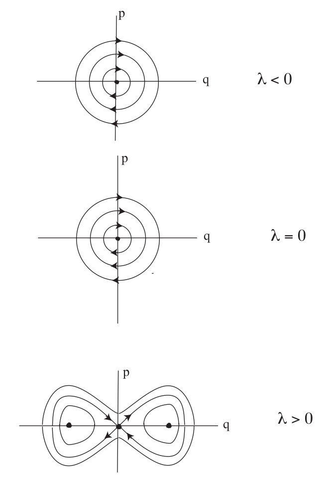
We consider the Hamiltonian:
H(q,p)=p22−λq22+q44,where λ is considered to be a parameter that can be varied. From this Hamiltonian, we derive Hamilton's equations:
˙q=∂H∂p=p,˙p=−∂H∂q=λq−q3.The fixed points for (7) are:
(q,p)=(0,0),(±√λ,0),from which it follows that there is one fixed point for λ≤0, and three fixed points for λ>0. This is the scenario for a pitchfork bifurcation.
Next we examine the stability of the fixed points. The Jacobian of (7) is given by:
J=(01λ−3q20).The eigenvalues of this matrix are:
Λ1,2=±√λ−3q2.Hence (q,p)=(0,0) is a center for λ<0, a saddle for λ>0 and has two zero eigenvalues for λ=0. The fixed points (q,p)=(√λ,0) are centers for λ>0. The phase portraits are shown in Fig. fig:2.