Two Degree-of-freedom de Leon-Berne Model

Introduction

Development of the Problem

We will consider the two degrees-of-freedom Hamiltonian for a unimolecular conformational isomerization introduced and studied extensively by De Leon and co-authors [1], [2], [3], [4], [5]. This 2 degrees-of-freedom Hamiltonian is given by H(x,y,px,py)=T(px,py)+VDB(x,y)=p2x2ms+p2y2ms+VDB(x,y)

where the potential energy function VDB(x,y) is (a detailed description is in the Appendix: [appsect:dbpot]{reference-type="ref" reference="appsect:dbpot"}) VDB(x,y)=Dx[1−exp(−λx)]2+V‡y4wy2(y2−2y2w)exp(−ζλx)+ϵs

and we will focus on varying λ and ζ.

The underlying Hamiltonian vector field is given by ˙x=∂H∂px=pxms˙y=∂H∂py=pyms˙px=−∂H∂x=2Dxλexp(−λx)(exp(−λx)−1)+V‡y4wζλy2(y2−2y2w)exp(−ζλx)˙py=−∂H∂y=−4V‡y4wy(y2−y2w)exp(−ζλx)

The total energy will be denoted by H(x,y,px,py)=E=Esaddle+ΔE where ΔE is the excess energy above the isomerization barrier energy.

The equilibrium points are located at ¯qs=(0,0,0,0) and at ¯qc=(xeq,±yw,0,0) where the x-coordinate, xeq, needs to be obtained using numerical root solver.

The total energy of the equilibrium point ¯qs is H(¯qs)=ϵs for all parameter values, and will be referred to as the critical energy. The total energy of the equilibrium point ¯qc is given by

H(¯qc)=Dx(1−exp(−λxeq))2−V‡exp(−ζλxeq)+ϵs

When ζ=0, the equilibrium point ¯qc is at (0,±yw,0,0), and has total energy ϵs−V‡ (see Supplemental material for details).

Potential energy function

VDB(x,y)=Dx[1−exp(−λx)]2+V‡y4wy2(y2−2y2w)exp(−ζλx)+ϵs

In this study, we fix μ=8,Dx=10,yw=1/√2,V‡=1,ϵs=1, and vary the parameters ζ,λ.

The equilibrium point is at (0,0,0,0) for all parameter values and the two equilibrium points are at (xeq,±yw,0,0) which needs to be calculated using a numerical root solver and depends on Dx,yw,V‡,ζ,λ. The equilibrium point at (0,0,0,0) has energy E(0,0,0,0)=ϵs. While the equilibrium point at (xeq,±yw,0,0) has total energy

The total energy of the equilibrium points at (xeq,±yw,0,0) is H(xeq,±yw,0,0)=E(xeq,±yw,0,0)=VDB(xeq,±yw,0,0)=Dx[1−exp(−λxeq)]2−V‡exp(−ζλxeq)+ϵs

\centering \subfigure[]{\includegraphics[width=0.32\textwidth]{./figures/pe_contour_param_fig3-A1}} \subfigure[]{\includegraphics[width=0.31\textwidth]{./figures/pe_contour_param_fig3-A2}} \

[[fig:pecontours_fig3db1981]]{#fig:pecontours_fig3db1981 label="fig:pecontours_fig3db1981"}

REPEATED SECTION

Two DoF de Leon-Berne system

We will consider the two degrees-of-freedom Hamiltonian for a unimolecular conformational isomerization introduced and studied extensively by De Leon and co-authors [1], [2], [3], [4], [5]. This 2 degrees-of-freedom Hamiltonian is given by \begin{aligned} \mathcal{H}(x,y,p_x,p_y) =& T(p_x, p_y) + V_{\rm DB}(x,y)  \\ =& \frac{p_x^2}{2m_s} + \frac{p_y^2}{2m_s} + V_{\rm DB}(x,y) \end{aligned} \label{eqn:ham_db}

where the potential energy function VDB(x,y) is (a detailed description is in the Appendix: [appsect:dbpot]{reference-type="ref" reference="appsect:dbpot"}) V_{\rm DB}(x,y) = D_x\left[ 1 - \exp(-\lambda x) \right]^2 + \dfrac{\mathcal{V}^{\ddagger}}{y_w^4}y^2(y^2 -  2y_w^2)\exp(-\zeta \lambda x) + \epsilon_s    \label{eqn:sys_pot}

and we will focus on varying λ and ζ.

The underlying Hamiltonian vector field is given by \begin{aligned} \dot{x} = \frac{\partial \mathcal{H}}{\partial p_x} &= \frac{p_x}{m_s} \\ \dot{y} = \frac{\partial \mathcal{H}}{\partial p_y} &=  \frac{p_y}{m_s}  \\ \dot{p_x} = - \frac{\partial \mathcal{H}}{\partial x}  &= 2 D_x \lambda \exp(-\lambda x)  (\exp(-\lambda x) - 1) + \\ & \qquad \dfrac{\mathcal{V}^{\ddagger}}{y_w^4}\zeta  \lambda y^2(y^2 - 2y_w^2)\exp(-\zeta \lambda x)\\ \dot{p_y} = -\frac{\partial \mathcal{H}}{\partial y} &=  -4  \dfrac{\mathcal{V}^{\ddagger}}{y_w^4}y(y^2 - y_w^2)\exp(- \zeta \lambda x) \end{aligned} \label{eqn:vec_field_db}

The total energy will be denoted by H(x,y,px,py)=E=Esaddle+ΔE where ΔE is the excess energy above the isomerization barrier energy.

The equilibrium points are located at ¯qs=(0,0,0,0) and at ¯qc=(xeq,±yw,0,0) where the x-coordinate, xeq, needs to be obtained using numerical root solver.

The total energy of the equilibrium point ¯qs is H(¯qs)=ϵs for all parameter values, and will be referred to as the critical energy. The total energy of the equilibrium point ¯qc is given by

H(¯qc)=Dx(1−exp(−λxeq))2−V‡exp(−ζλxeq)+ϵs

When ζ=0, the equilibrium point ¯qc is at (0,±yw,0,0), and has total energy ϵs−V‡ (see Supplemental material for details).

{width="33.0000%"}\ {width="33.0000%"}\ {width="33.0000%"} [[fig:pecontours_db]]

Fig. 1. Potential energy function for the De Leon-Berne model of unimolecular isomerization for 3 different sets of coupling and range parameters used in~\citeauthor{de_leon_intramolecular_1981}~\cite{de_leon_intramolecular_1981}. It is to be noted that the potential energy surface is ``mostly'' flat and then becomes steep for large x<0. The coordinates of the saddle equilibrium point are also independent of the parameters and located at the origin.

REPEATED SECTION

Revealing the phase space structure

Invariant manifolds and unstable periodic orbits {#sect:tubes_transition}

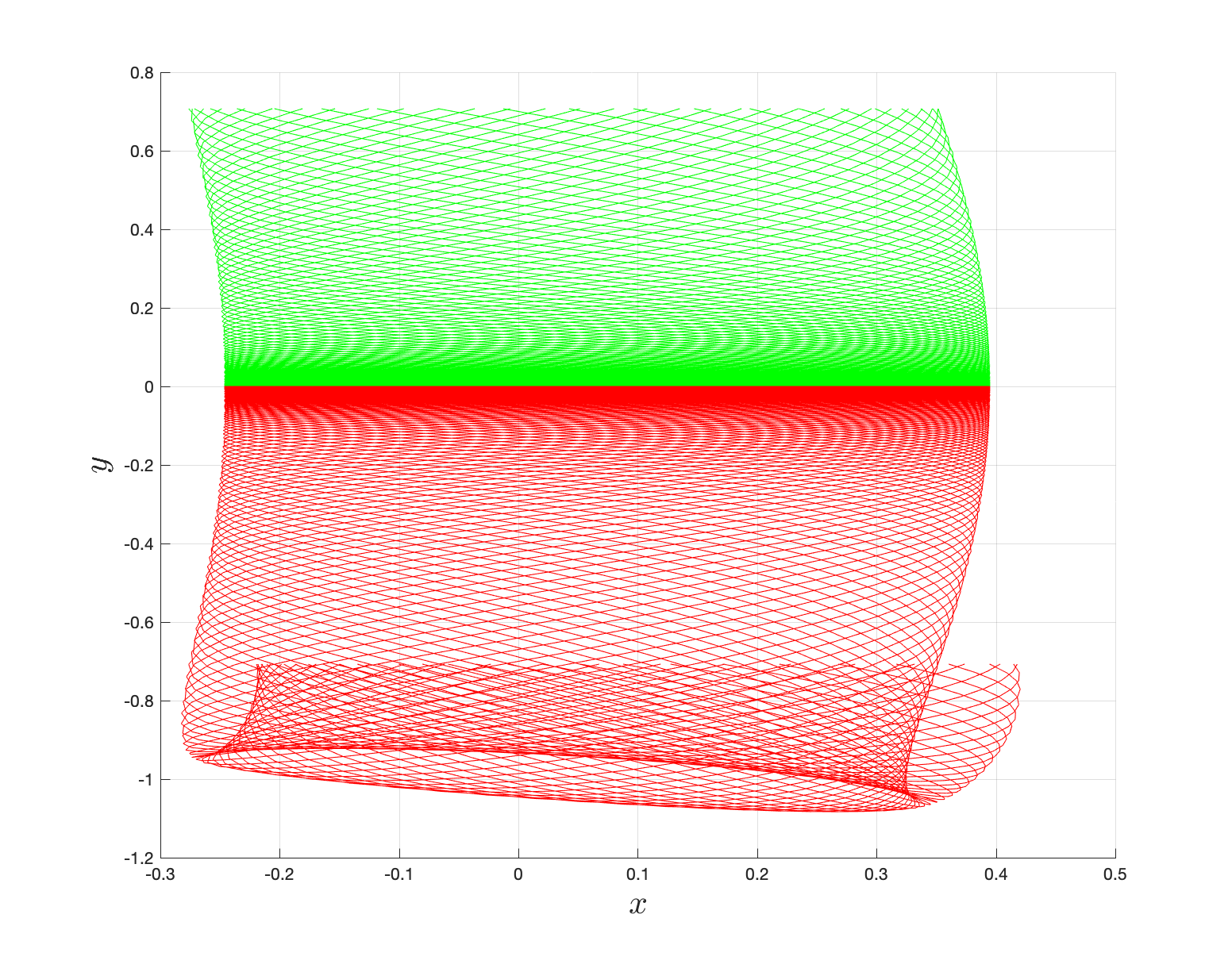
We consider the dynamics of conservative system by determining the phase space "skeleton" that governs transition between potential well (or, equivalently escape from a well). In the simplest case of only two degrees of freedom, the phase space is of 4 dimensional and the boundary between potential wells is defined using unstable periodic orbit that lie in the bottleneck connecting the wells. The set of all states leading to escape from a potential well can be understood as residing within an invariant manifold of geometry R1×S1, that is a cylinder or tube. The interior of this tube defines the set of all states which will transition to the adjacent well.

Linearization near the rank-1 saddle

It is to be noted that the linearization of the behavior of trajectories near the saddle-center equilibrium points appears in the leading order expression of the transition fraction. We are interested in trajectories which have an energy just above that of the critical value. The region of possible motion for E>Ec contains a neck around each saddle equilibrium point. The geometry of trajectories close to the neck region is studied by considering the linearized equations of motion near the equilibrium point.

In this section, let xeq denote the equilibrium point connecting the top and bottom wells. Furthermore, for a fixed energy E, we consider a neighborhood of xeq on the energy surface, whose configuration space projections are the bottleneck regions. We refer to this neighborhood as the equilibrium region and denote it by R on the energy surface. We perform a coordinate transformation with xeq=(xeq,yeq,0,0) as the new origin, and keep the first order terms, we obtain ˙x=J(xeq)xwhere,x=[x,y,px,py]T

where J(xe,1) is the Jacobian of the Hamiltonian vector field [eqn:vec_field_db]{reference-type="eqref" reference="eqn:vec_field_db"} evaluated at the equilibrium point. The Jacobian involves derivatives of Eqns. [eqn:pot_energy_db]{reference-type="eqref" reference="eqn:pot_energydb"} and the kinetic energy does not depend on the position coordinates, we can write compactly $$\begin{aligned} \mathbb{J}(\mathbf{x}) = D\mathbf{f}(\mathbf{x}) = (001/μ00001/μ−∂2H∂x2−∂2H∂y∂x00−∂2H∂x∂y−∂2H∂y200)

= \ \begin{pmatrix} 0 & 0 & 1/\mu & 0 \ 0 & 0 & 0 & 1/\mu \ -\frac{\partial^2 V{DB}}{\partial x^2} & -\frac{\partial^2 V{DB}}{\partial y \partial x} & 0 & 0 \ -\frac{\partial^2 V{DB}}{\partial x \partial y} & -\frac{\partial^2 V_{DB}}{\partial y^2} & 0 & 0 \end{pmatrix} \label{eqn:jacobian}\end{aligned}$$

Thus, the linearized vector field at the equilibrium point becomes ˙x=J(xeq)x=Df(xeq)=(001/μ00001/μ−2Dxλ20000800)x

where f denotes the Hamiltonian vector field. which has eigenvalues of the form λ,−λ,iω,−iω given by −√2ϵμA,√2ϵμA,i√2Dxmλ,−i√2Dxmλ,

and λ>0,ω>0, and corresponding eigenvectors given by uλ=[0,1,0,A√2ϵμ]u−λ=[0,1,0,−A√2ϵμ]uiω=[1,0,iλ√2Dxm,0]u−iω=[1,0,−iλ√2Dxm,0] Thus, the general (real) solution of [eqn:lin_sys_eqpt]{reference-type="eqref" reference="eqn:lin_sys_eqpt"} has the form x(t)=(x(t),y(t),px(t),py(t))=α1eλtuλ+α2e−λtu−λ+2Re(βeiωtuiω) where, α1, α2 are real and β=β1+iβ2 is complex.

Numerical method for computing reactive islands

Step 1: Select appropriate energy above the critical value  For computing the unstable periodic orbits and its invariant manifolds that are phase space conduits for transition between the two isomers, we have to specify a total energy, E, that is above the energy of the index-1 saddle (this is referred to as critical energy or reference energy or isomerization energy, Ec, in the chemical reaction dynamics literature) and so the excess energy ΔE=E−Ec>0. This excess energy can be arbitrarily large as long as the unstable periodic orbit does not bifurcate.

Step 2: Compute the unstable periodic orbit associated with the rank-1 saddle  We consider a procedure which computes unstable periodic orbits associated with rank-1 saddle in a straightforward fashion. This procedure begins with small "seed" initial conditions obtained from the linearized equations of motion near xeq, and uses differential correction and numerical continuation to generate the desired periodic orbit corresponding to the chosen energy E [6]. The result is a periodic orbit of the desired energy E of some period T, which will be close to 2π/ω where ±ω is the imaginary pair of eigenvalues of the linearization around the saddle point.

Guess for initial condition of a periodic orbit   The general solution of linearized equations of motion (Eqn. [eqn:linearSol]{reference-type="eqref" reference="eqn:linearSol"}) at the equilibrium point xeq can be used to initialize a guess for an iterative correction procedure called differential correction. The linearization yields an eigenvalue problem Av=γv, where A is the Jacobian matrix evaluated at the equilibrium point, γ is the eigenvalue, and v=[k1,k2,k3,k4]T is the corresponding eigenvector. We initialize the guess for the periodic orbit for a small amplitude, Ax<<1. Let β=−Ax/2 and using the eigenvector spanning the center subspace, we can guess the initial condition to be ˉx(0)=ˉx0,g=(x0,g,y0,g,px0,g,py0,g)T=(xeq,yeq,0,0)T+2Re(βuiω)=(xeq−Ax,yeq,0,0)T

Differential correction of the initial condition  In this iterative correction procedure, we introduce small change in the guess for the initial condition such that coordinates at the final and initial time of the periodic orbit ‖ˉxpo(T)−ˉxpo(0)‖<ϵ

for some tolerance ϵ<<1. In this approach, we hold x−coordinate constant, while applying correction to the initial guess of the y−coordinate, use px−coordinate for terminating event-based integration, and py−coordinate to test convergence of the periodic orbit. It is to be noted that a specific combination of the phase space coordinates is only suitable for potential, and in general will require some permutation of the coordinates to achieve a stable algorithm.

Let us denote the flow map of a differential equation ˚x=f(x) with an initial condition x(t0)=x0 by ϕ(t;x0). Thus, the displacement of the final state under a perturbation δt becomes δˉx(t+δt)=ϕ(t+δt;ˉx0+δˉx0)−ϕ(t;ˉx0)

with respect to the reference orbit ˉx(t). Thus, measuring the displacement at t1+δt1 and expanding into Taylor series gives δˉx(t1+δt1)=∂ϕ(t1;ˉx0)∂x0δˉx0+∂ϕ(t1;ˉx0)∂t1δt1+h.o.t where the first term on the right hand side is the state transition matrix, Φ(t1,t0), when δt1=0. Thus, it can be obtained as numerical solution to the variational equations as discussed in [7]. Let us suppose we want to reach the desired point xd, we have ˉx(t1)=ϕ(t1;ˉx0)=ˉx1=xd−δˉx1 which has an error δˉx1 and needs correction. This correction to the first order can be obtained from the state transition matrix at t1 and an iterative procedure of this small correction based on first order yields convergence in few steps. For the equilibrium point under consideration, we initialize the guess as ˉx(0)=(x0,g,y0,g,px0,g,py0,g)T=(−Ax,0,0,0)T and using numerical integrator we continue until next px=0 event crossing with a high specified tolerance (typically 10−14). So, we obtain ˉx(t1) which for the guess periodic orbit denotes the half-period point, t1=T0,g/2 and compute the state transition matrix Φ(t1,0). This can be used to correct the initial value of y0,g to approximate the periodic orbit while keeping x0,g constant. Thus, correction to the first order is given by δpx1=Φ32δy0+˚px1δt1+h.o.tδpy1=Φ42δy0+˚py1δt1+h.o.t where Φij is the (i,j)th entry of Φ(t1,0) and the acceleration terms come from the equations of motion evaluated at the crossing t=t1 when px1=δpx1=0. Thus, we obtain the first order correction δy0 as δy0≈(Φ42−Φ32˚py1˚px1)−1δpy1y0→y0−δy0 which is iterated until |py1|=|δpy1|<ϵ for some tolerance ϵ, since we want the final periodic orbit to be of the form ˉxt1=(x1,y1,0,0)T

This procedure yields an accurate initial condition for a periodic orbit of small amplitude Ax<<1, since our initial guess is based on the linear approximation near the equilibrium point. It is also to be noted that differential correction assumes the guess periodic orbit has a small error (for example in this system, of the order of 10−2) and can be corrected using first order form of the correction terms. If, however, larger steps in correction are applied this can lead to unstable convergence as the half-orbit overshoots between successive steps. Even though there are other algorithms for detecting unstable periodic orbits, differential correction is easy to implement and shows reliable convergence for generating a dense family of periodic orbits (UPOs) associated with the rank-1 saddle at arbitrary high excess energy (as long as UPOs don't bifurcate). These unstable perioidic orbit at high excess energy are required for constructing codimension−1 invariant manifolds.

Numerical continuation to periodic orbit at arbitrary energy  The above procedure yields an accurate initial condition for a unstable periodic orbit from a single initial guess. If our initial guess came from the linear approximation near the equilibrium point, from Eqn. [eqn:linearSol]{reference-type="eqref" reference="eqn:linearSol"}, it has been observed in the numerics that we can only use the differential correction procedure for small amplitude (∼10−4) periodic orbit around xe. This small amplitude corresponds to small excess energy, typically ∼10−2, and to find an unstable periodic orbit of arbitrarily large amplitude, we resort to the procedure of numerical continuation to generate a family which reaches the appropriate energy E. Numerical continuation uses the two small amplitude periodic orbits obtained from the differential correction procedure and proceeds as follows.

Suppose we find two small nearby periodic orbit initial conditions, ˉx(1)0 and ˉx(2)0, correct to within the tolerance d, using the differential correction procedure described above. We can then generate a family of periodic orbits with successively increasing amplitudes associated with the rank-1 saddle ˉxe in the following way. Let Δ=ˉx(2)0−ˉx(1)0=[Δx0,Δy0,0,0]T

A linear extrapolation to an initial guess of slightly larger amplitude, ˉx(3)0 is given by ˉx(3)0,g= ˉx(2)0+Δ=[(x(2)0+Δx0),(y(2)0+Δy0),0,0]T=[x(3)0,y(3)0,0,0]T Now, we can use differential correction to refine the guess initial condition ˉx(3)0,g until a specified tolerance is satisfied. Then, we repeat using ˉx(3)0 and ˉx(2)0 to obtain the next ˉx(4)0, so on and so forth until we have a family of solutions. We can keep track of the energy of each periodic orbit and when we have two solutions, ˉx(k)0 and ˉx(k+1)0, whose energy bisects the desired target energy, Etarget, we halt the numerical continuation of the family. Next, we resort to combining bisection and differential correction to the last two periodic orbits until we converge to the unstable periodic orbit at Etarget to within a specified tolerance. Thus, the result is a periodic orbit at Etarget and of some period Tpo with an initial condition ˉx0.

Step 3: Computation of invariant manifolds. First, we find the local approximation to the unstable and stable manifolds of the periodic orbit from the eigenvectors of the monodromy matrix. Next, the local linear approximation of the unstable (or stable) manifold in the form of a state vector is integrated in the nonlinear equations of motion to produce the approximation of the unstable (or stable) manifolds. This procedure is known as globalization of the manifolds and we proceed as follows

First, the state transition matrix Φ(t) along the periodic orbit with initial condition ˉx0 can be obtained numerically by integrating the variational equations along with the equations of motion from t=0 to t=T. This is known as the monodromy matrix M=Φ(T) and the eigenvalues can be computed numerically. The theory for Hamiltonian systems (see Ref. [8] for details) tells us that the four eigenvalues of M are of the form λ1>1,λ2=1λ1,λ3=λ4=1

The eigenvector associated with eigenvalue λ1 is in the unstable direction, the eigenvector associated with eigenvalue λ2 is in the stable direction. Let es(ˉx0) denote the normalized (to 1) stable eigenvector, and eu(ˉx0) denote the normalized unstable eigenvector. We can compute the stable manifold and unstable manifold at ˉx0 by initializing along the eigenvectors Xs/u(ˉx0)=ˉx0+ϵes/u(ˉx0). Here the small displacement from ˉx0 is denoted by ϵ and its magnitude should be small enough to be within the validity of the linear estimate, yet not so small that the time of flight becomes too large due to asymptotic nature of the stable and unstable manifolds. Ref. [6] suggests typical values of ϵ>0 corresponding to nondimensional position displacements of magnitude around 10−6. By numerically integrating the unstable vector forwards in time, using both ϵ and −ϵ, for the two branches emanating from the NHIM, respectively, we generate trajectories shadowing the two branches, Wu+ and Wu−, of the unstable manifold of the NHIM. Similarly, by integrating the stable vector backwards in time, using both ϵ and −ϵ, for forward and backward branch respectively, we generate trajectories shadowing the stable manifold, Ws+,−. For the manifold at X(t), one can simply use the state transition matrix to transport the eigenvectors from X0 to X(t): Xs/u(X(t))=Φ(t,0)Xs/u(ˉx0) It is to be noted that since the state transition matrix does not preserve the norm and so the resulting vector must be normalized. The globalized invariant manifolds associated with rank-1 saddles are known as Conley-McGehee tubes and these spherical cylinders form the impenetrable barriers and phase space conduits for transition between potential wells (missing reference).

Step 4: Reactive islands and committor probabilities In Ref. (missing reference), the authors discussed the role of reactive islands (RI) in sampling a rare trajectory and the sensitivity of the committor probability to the geometry of the RI structure.

Implications for Reaction Dynamics

Direct numerical computation of reactive islands

{width="45%"}\ 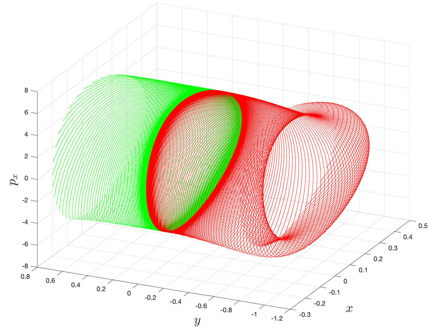{width="45%"}

Fig. 2. Tube manifolds for the coupled system ζ=1.00 and λ=1.50

Connecting hierarchy of reactive islands with committor probabilities: Lagrangian descriptor

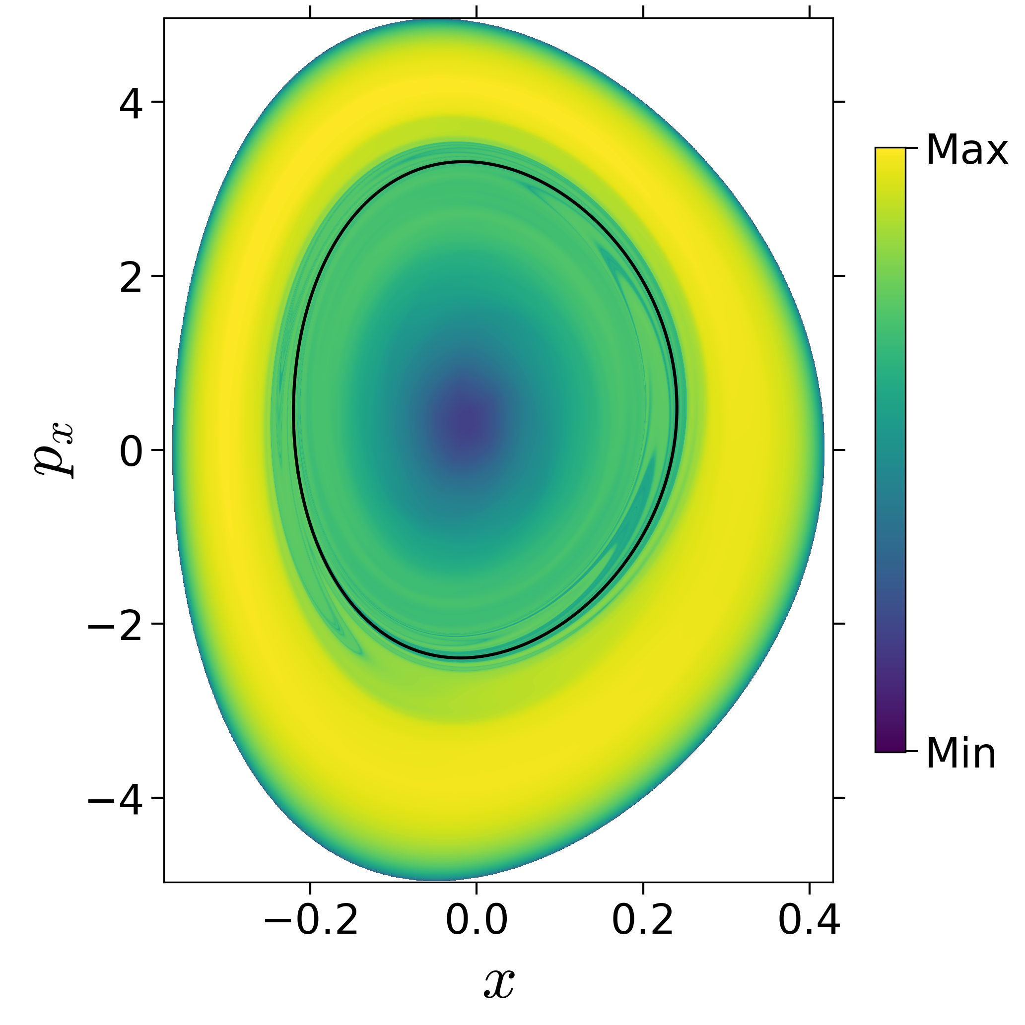
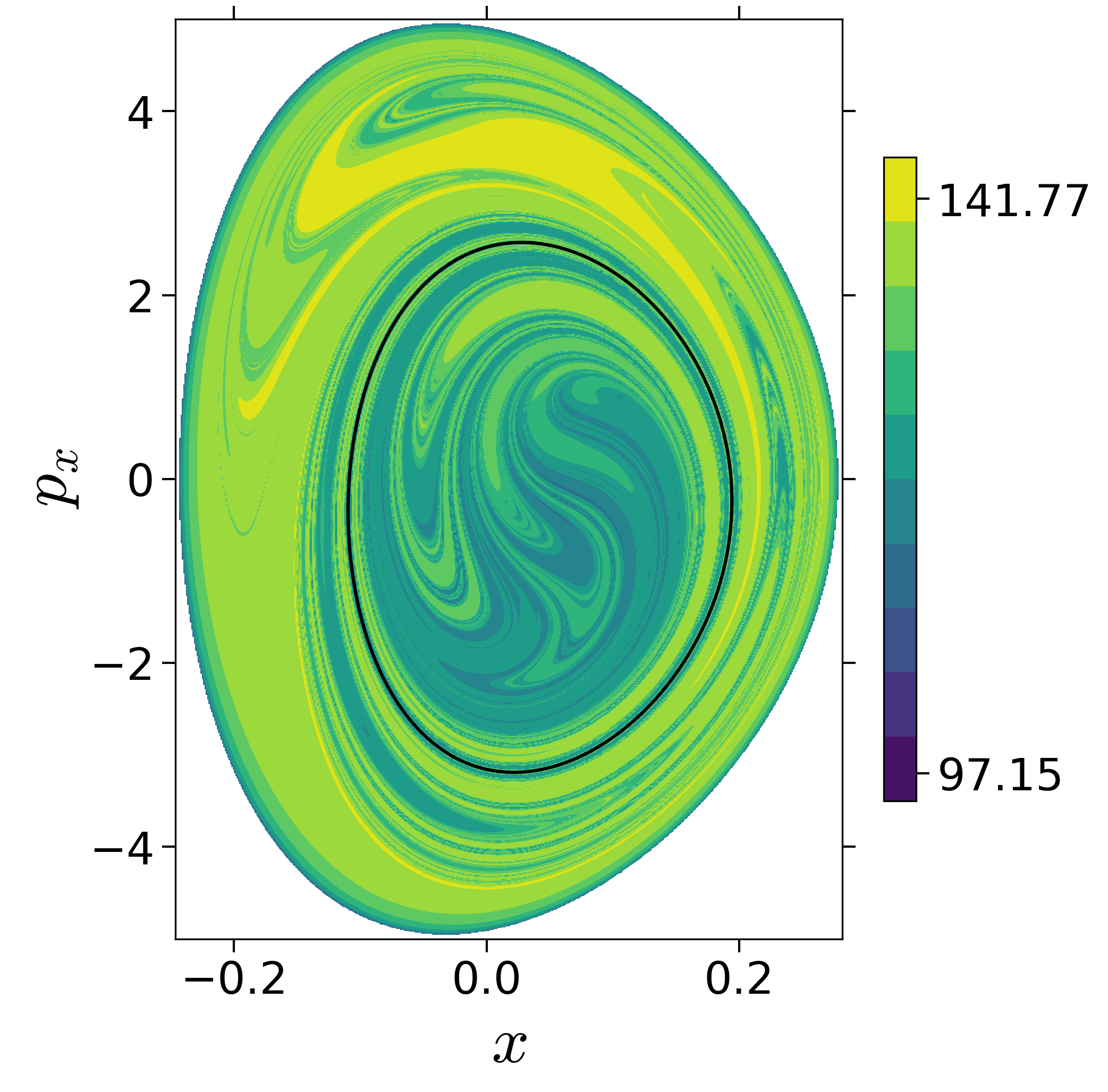
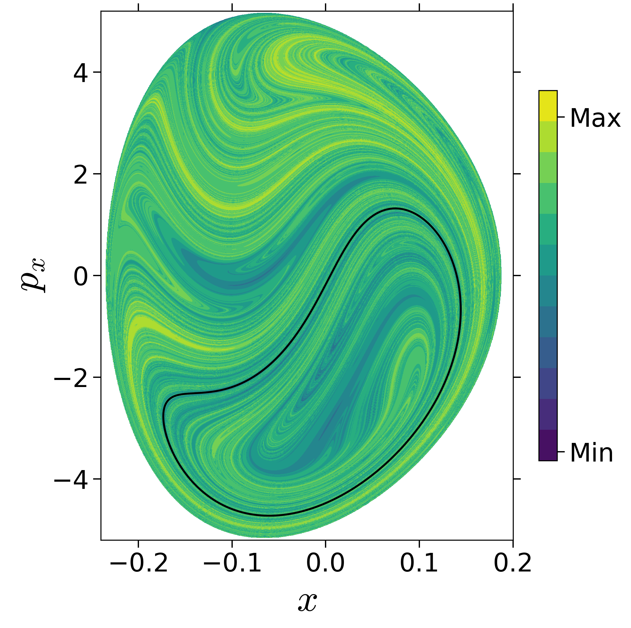
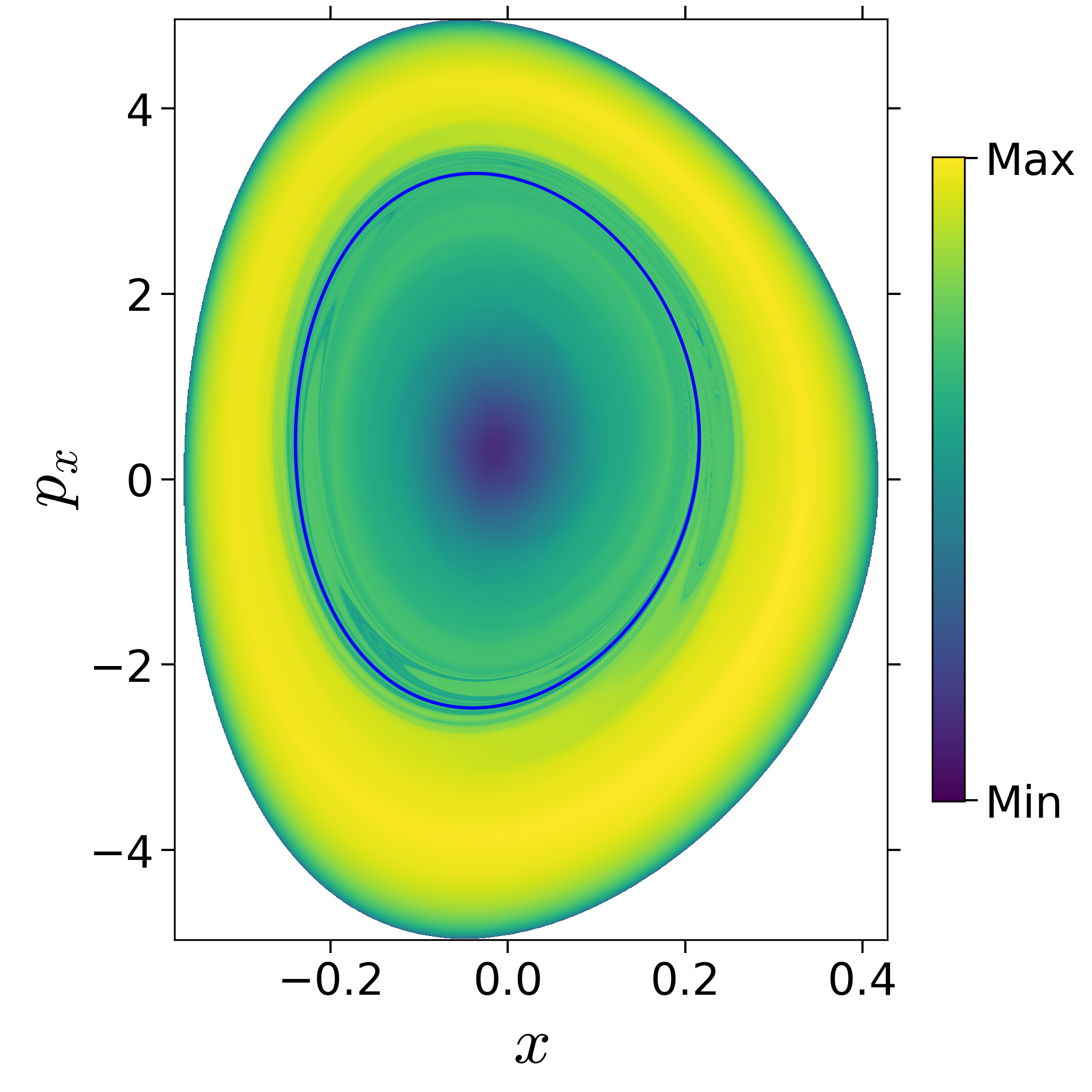
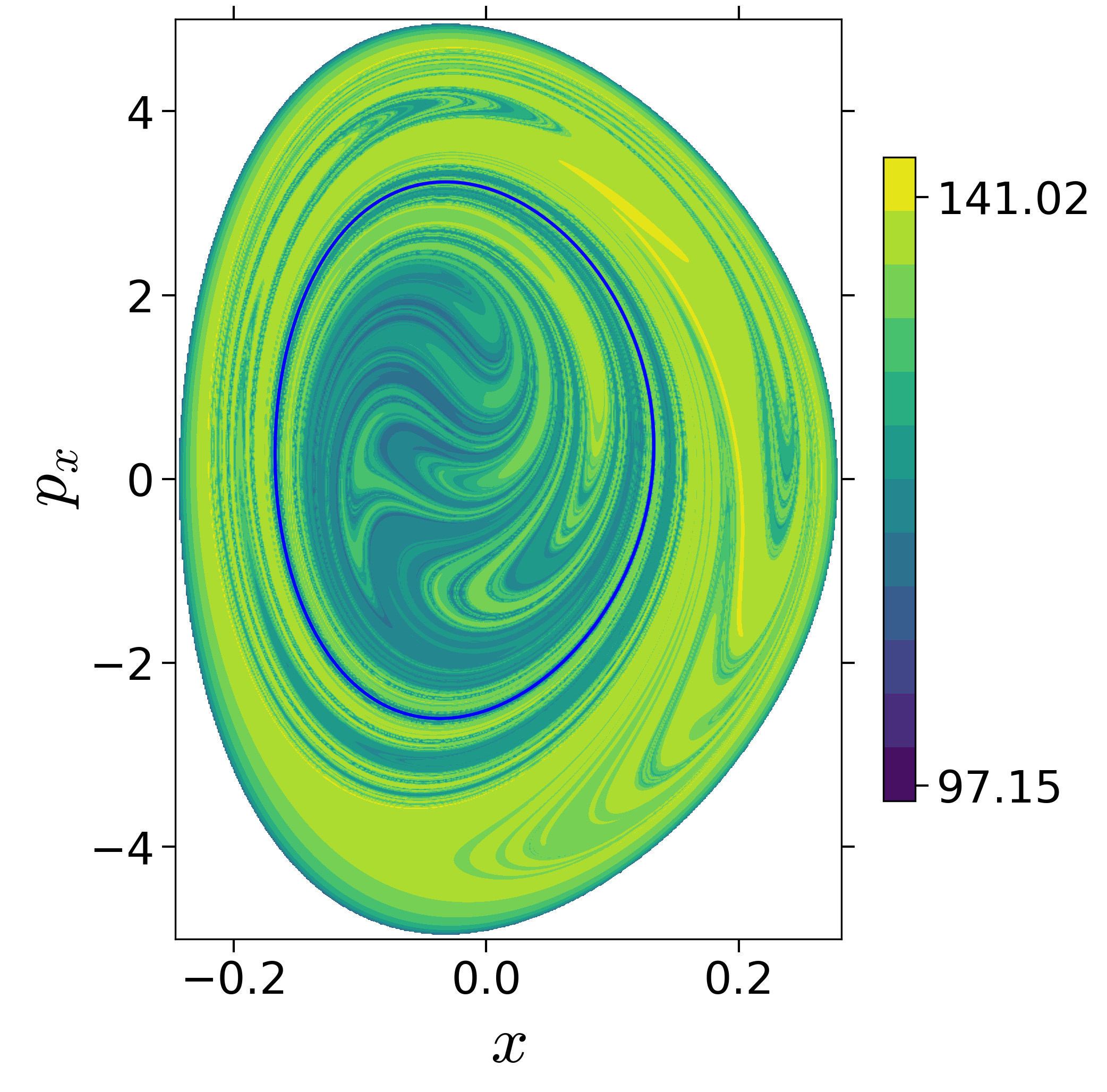
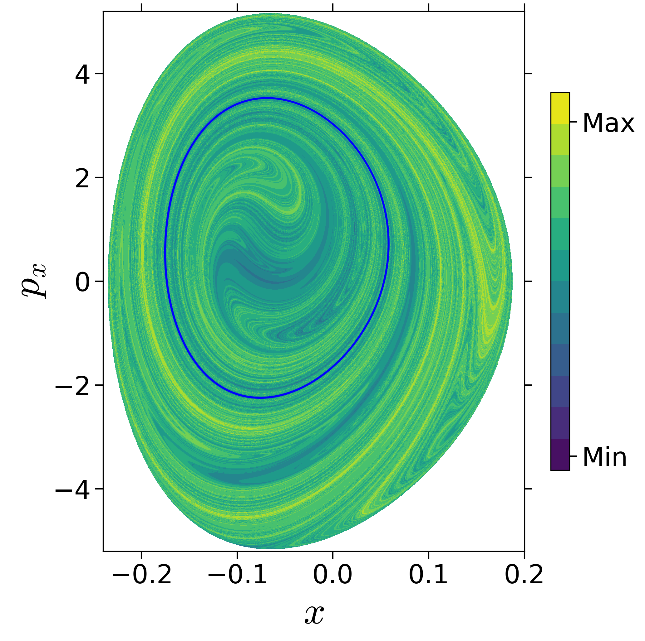
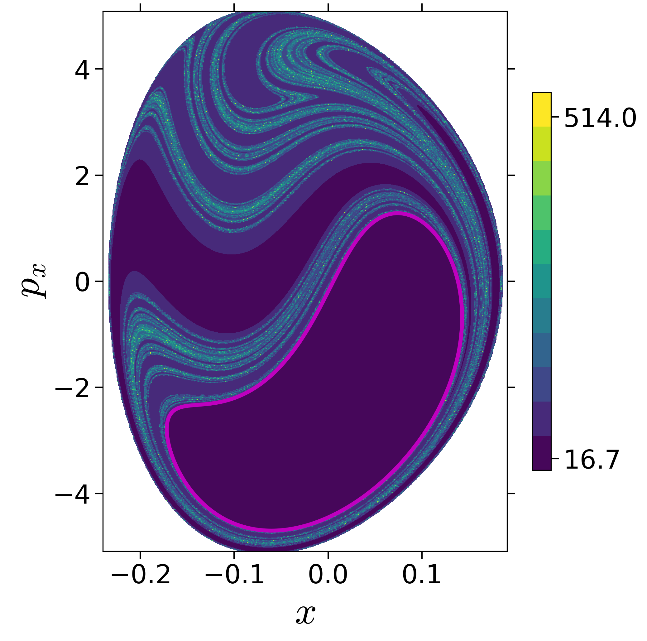
Finding reactive islands in 2 degrees-of-freedom molecular Hamiltonian has been shown using Lagrangian descriptors [9], [10].

First, we will use the following 2D isonergetic slice to compute Lagrangian descriptor contour map so that the reactive islands can be identified.

U−xpx={(x,y,px,py)|y=yw,py(x,y,px;E)<0}

for 4 cases of coupling and range parameters, ζ and λ. However, we will choose the system parameters: ζ=1.00,λ=1.50 and ζ=2.30,λ=1.95 as representative of regular and chaotic dynamics of the isomerization in the gas phase.

{width="25%"}\ {width="25%"}\ {width="25%"}\ {width="25%"}\ {width="25%"}\ {width="25%"}\

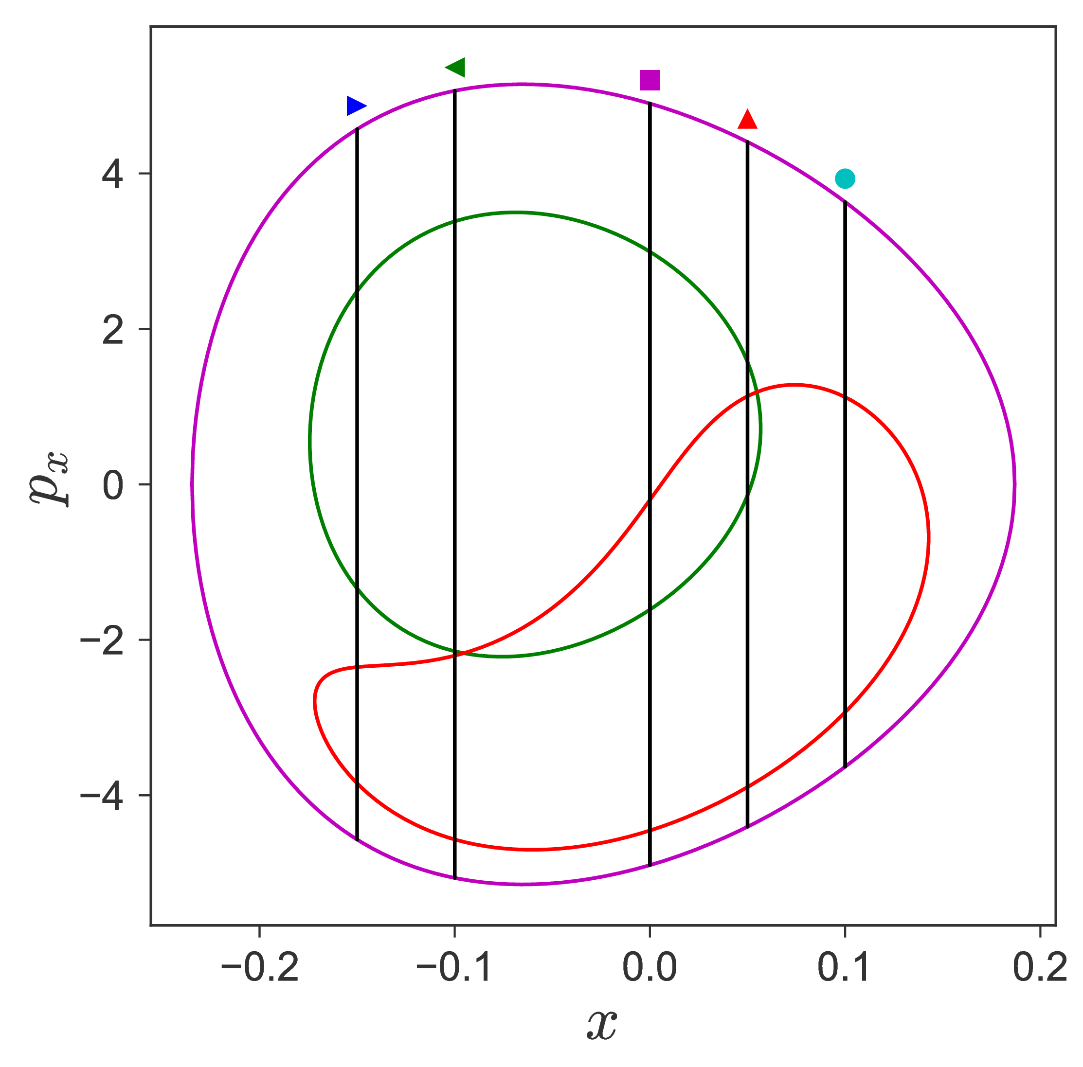
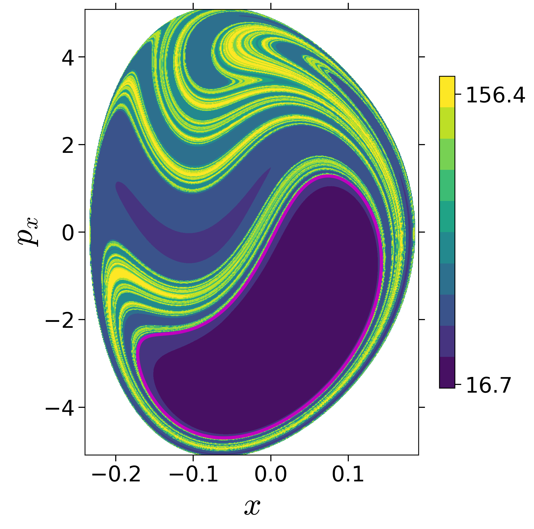
Fig. 3. Lagrangian descriptor and reactive islands for (a,d) ζ=1.00 and λ=1.00, (b,e) ζ=1.00 and λ=1.50, (c,f) ζ=2.30 and λ=1.95. The top row shows the backward LD and the bottom row shows the forward LD. The blue and black curves denote the intersection of stable and unstable manifolds with the surface-of-section, respectively, and integration time τ=30 and microcanonical ensemble of trajectories are initialized on the surface of section~(???).

In transition path sampling, the method to check the efficiency of the sampling procedure is done by computing the committor probability of starting in region A and ending up in region B (A and B are defined in the configuration space) for the configuration qj denoted by the PB(qj,tc) [11], [9]. This is defined as the fraction of the trajectories that reach the specific product in region B at time tc before reaching reactant in region A. For the unimolecular conformational isomerization, the region A and B are defined by the isomers A and B, respectively, while the specific reactant and product configuration is defined by the parameter yw.

{width="25%"}

{width="24%"}\ 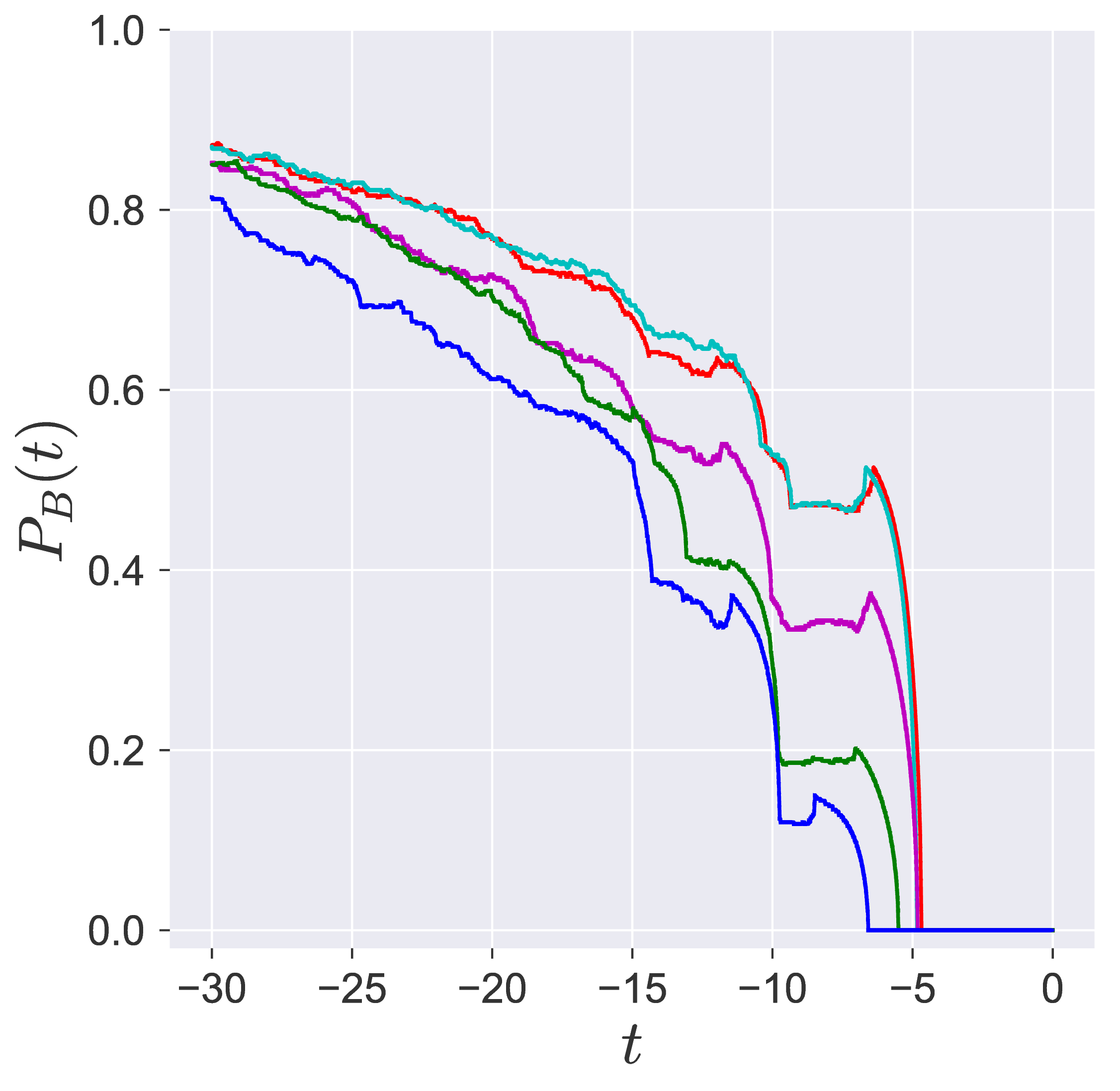{width="24%"}\ 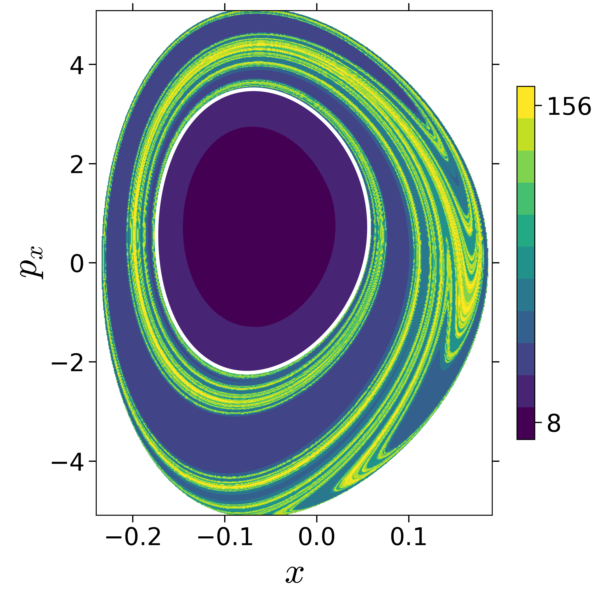{width="24%"}\ 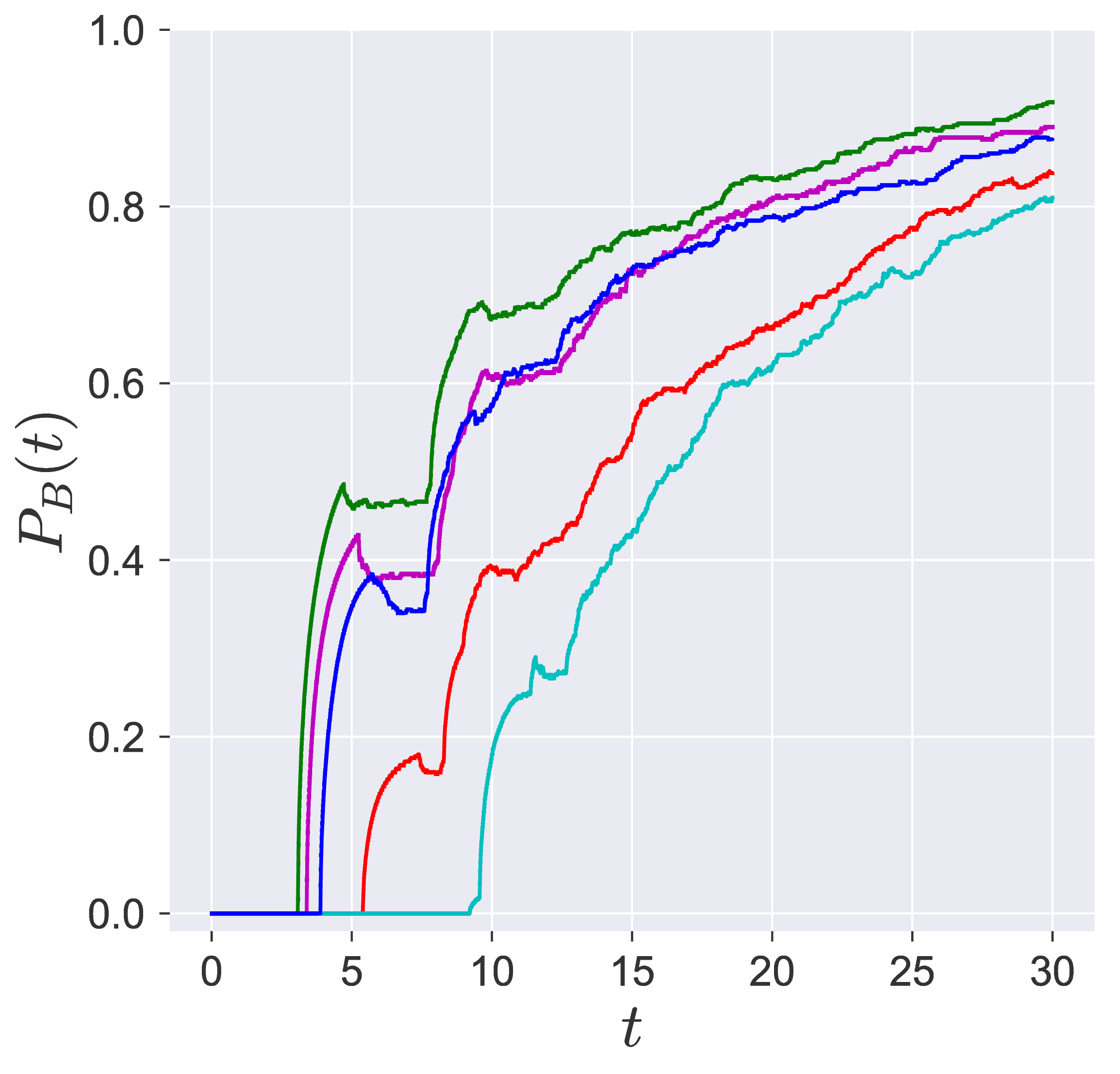{width="24%"}

{width="24%"}\ 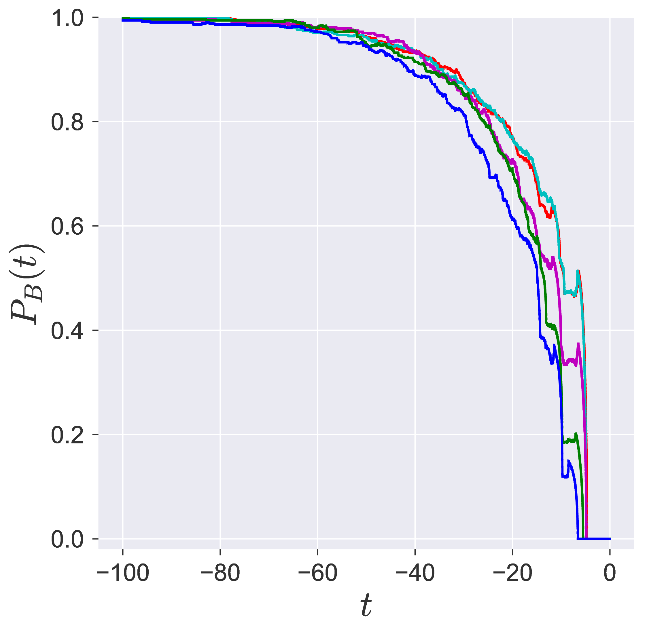{width="24%"}\ 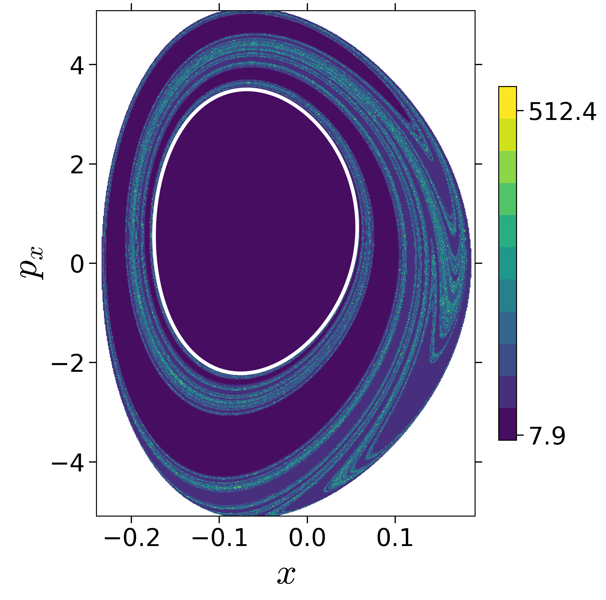{width="24%"}\ 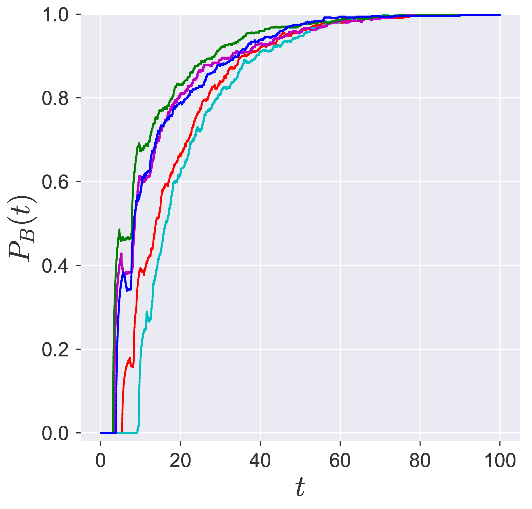{width="24%"}

Fig. 4. Committor probabilities and reactive islands for the 2 DoF isomerization. (a) Reactive islands obtained using direct computation of the cylindrical manifolds. (b-e) τ=30: color maps denote variable integration time LDs and the line plots denote the committor probabilities. (f-i) τ=100: color maps denote variable integration time LDs and the line plots denote the committor probabilities. Coupling strength, ζ=2.30, and Morse range, λ=1.95.

Probability of imminent reaction

The area enclosed by the stable or unstable manifolds of the unstable periodic orbit associated with the index-1 saddle is used to calculate the reacting population of trajectories at a constant total energy E. This population will be referred to as the microcanonical reaction probability.

For a systematic detection of the trajectories that lead to reaction by crossing the unstable periodic orbit in the bottleneck, we enforce the sign of momentum of these trajectories. So a positive ˙y=py<0 on the surface-of-section y=yw denotes crossing the

The fraction of trajectories that cross the section at y=yw in forward and backward time are unstable periodic orbit located in the bottleneck

\centering {width="49%"} {width="49%"}

Additional slices of Lagrangian descriptor

U+xpx={(x,y,px,py)|y=1/√2,py(x,y,px;e)<0}

\centering \subfigure[]{\includegraphics[width=0.24\textwidth]{./figures/fig3A2/backward_lag_desc_deleonberne_E1-510_x-px_tau30.png}} \subfigure[]{\includegraphics[width=0.24\textwidth]{./figures/fig3A2/backward_lag_desc_deleonberne_E3-000_x-px_tau30.png}} \subfigure[]{\includegraphics[width=0.24\textwidth]{./figures/fig3A2/backward_lag_desc_deleonberne_E4-500_x-px_tau30.png}} \subfigure[]{\includegraphics[width=0.24\textwidth]{./figures/fig3A2/backward_lag_desc_deleonberne_E6-000_x-px_tau30.png}} \subfigure[]{\includegraphics[width=0.24\textwidth]{./figures/fig3A2/forward_lag_desc_deleonberne_E1-510_x-px_tau30.png}} \subfigure[]{\includegraphics[width=0.24\textwidth]{./figures/fig3A2/forward_lag_desc_deleonberne_E3-000_x-px_tau30.png}} \subfigure[]{\includegraphics[width=0.24\textwidth]{./figures/fig3A2/forward_lag_desc_deleonberne_E4-500_x-px_tau30.png}} \subfigure[]{\includegraphics[width=0.24\textwidth]{./figures/fig3A2/forward_lag_desc_deleonberne_E6-000_x-px_tau30.png}} \centering \subfigure[]{\includegraphics[width=0.24\textwidth]{./figures/fig3B2/backward_lag_desc_deleonberne_E3-000_x-px_tau30.png}} \subfigure[]{\includegraphics[width=0.24\textwidth]{./figures/fig3B2/backward_lag_desc_deleonberne_E4-500_x-px_tau30.png}} \

\centering \subfigure[]{\includegraphics[width=0.24\textwidth]{./figures/fig3C2/backward_lag_desc_deleonberne_E1-510_x-px_tau30.png}} \subfigure[]{\includegraphics[width=0.24\textwidth]{./figures/fig3C2/backward_lag_desc_deleonberne_E3-000_x-px_tau30.png}} \subfigure[]{\includegraphics[width=0.24\textwidth]{./figures/fig3C2/backward_lag_desc_deleonberne_E4-500_x-px_tau30.png}} \subfigure[]{\includegraphics[width=0.24\textwidth]{./figures/fig3C2/backward_lag_desc_deleonberne_E7-000_x-px_tau30.png}} \subfigure[]{\includegraphics[width=0.24\textwidth]{./figures/fig3C2/forward_lag_desc_deleonberne_E1-510_x-px_tau30.png}} \subfigure[]{\includegraphics[width=0.24\textwidth]{./figures/fig3C2/forward_lag_desc_deleonberne_E3-000_x-px_tau30.png}} \subfigure[]{\includegraphics[width=0.24\textwidth]{./figures/fig3C2/forward_lag_desc_deleonberne_E4-500_x-px_tau30.png}} \subfigure[]{\includegraphics[width=0.24\textwidth]{./figures/fig3C2/forward_lag_desc_deleonberne_E7-000_x-px_tau30.png}} Observation: within the τ=20 time interval unstable manifold for the second case has not fully intersected the surface-of-section.

U−ypy={(x,y,px,py)|x=0,px(x,y,py;E)<0}

\centering \subfigure[]{\includegraphics[width=0.24\textwidth]{./figures/fig3C2/backward_lag_desc_deleonberne_E1-500_y-py_tau30.png}} \subfigure[]{\includegraphics[width=0.24\textwidth]{./figures/fig3C2/backward_lag_desc_deleonberne_E3-000_y-py_tau30.png}} \subfigure[]{\includegraphics[width=0.24\textwidth]{./figures/fig3C2/backward_lag_desc_deleonberne_E4-500_y-py_tau30.png}} \subfigure[]{\includegraphics[width=0.24\textwidth]{./figures/fig3C2/backward_lag_desc_deleonberne_E6-000_y-py_tau30.png}} \subfigure[]{\includegraphics[width=0.24\textwidth]{./figures/fig3C2/forward_lag_desc_deleonberne_E1-500_y-py_tau30.png}} \subfigure[]{\includegraphics[width=0.24\textwidth]{./figures/fig3C2/forward_lag_desc_deleonberne_E3-000_y-py_tau30.png}} \subfigure[]{\includegraphics[width=0.24\textwidth]{./figures/fig3C2/forward_lag_desc_deleonberne_E4-500_y-py_tau30.png}} \subfigure[]{\includegraphics[width=0.24\textwidth]{./figures/fig3C2/forward_lag_desc_deleonberne_E6-000_y-py_tau30.png}}

\begingroup \bibliographystyle{rsc} \endgroup

References

1. N. De Leon and B. J. Berne, “Intramolecular rate process: Isomerization dynamics and the transition to chaos,” The Journal of Chemical Physics, vol. 75, no. 7, pp. 3495–3510, Oct. 1981.
2. N. De Leon and C. C. Marston, “Order in chaos and the dynamics and kinetics of unimolecular conformational isomerization,” The Journal of Chemical Physics, vol. 91, no. 6, pp. 3405–3425, Sep. 1989.
3. A. M. Ozorio de Almeida, N. De Leon, M. A. Mehta, and C. C. Marston, “Geometry and dynamics of stable and unstable cylinders in Hamiltonian systems,” Physica D: Nonlinear Phenomena, vol. 46, no. 2, pp. 265–285, 1990.
4. N. De Leon, M. A. Mehta, and R. Q. Topper, “Cylindrical manifolds in phase space as mediators of chemical reaction dynamics and kinetics. I. Theory,” The Journal of Chemical Physics, vol. 94, no. 12, pp. 8310–8328, Jun. 1991.
5. N. De Leon, “Cylindrical manifolds and reactive island kinetic theory in the time domain,” The Journal of Chemical Physics, vol. 96, no. 1, pp. 285–297, Jan. 1992.
6. W. S. Koon, M. W. Lo, J. E. Marsden, and S. D. Ross, Dynamical systems, the three-body problem and space mission design. Marsden books, 2011, p. 327.
7. T. S. Parker and L. O. Chua, Practical Numerical Algorithms for Chaotic Systems. New York, NY, USA: Springer-Verlag New York, Inc., 1989.
8. K. R. Meyer, G. R. Hall, and D. Offin, Introduction to Hamiltonian Dynamical Systems and the N-Body Problem. Springer, 2009.
9. S. Patra and S. Keshavamurthy, “Detecting reactive islands using Lagrangian descriptors and the relevance to transition path sampling,” Physical Chemistry Chemical Physics, vol. 20, no. 7, pp. 4970–4981, 2018.
10. S. Naik and S. Wiggins, “Finding normally hyperbolic invariant manifolds in two and three degrees of freedom with Hénon-Heiles-type potential,” Phys. Rev. E, vol. 100, no. 2, p. 022204, 2019.
11. P. G. Bolhuis, D. Chandler, C. Dellago, and P. L. Geissler, “Transition Path Sampling: Throwing Ropes Over Rough Mountain Passes, in the Dark,” Annual Review of Physical Chemistry, vol. 53, no. 1, pp. 291–318, 2002.