The one Degree-of-Freedom Morse Oscillator

Introduction and Development of the Problem

The potential energy function derived by P. M. Morse is truly a ''workhorse'' potential energy function in theoretical chemistry [1]. Originally it was devised to describe the intermolecular force between the two atoms in a diatomic molecule. It has the functional form:

\begin{equation} V(q) = D \left( 1-e^{-\alpha q} \right)^2, \label{eq:mpot} \end{equation}

where $q$ represents the distance between the two atoms, $D >0$ represents the depth of the potential well (defined relative to the dissociated atoms), and $\alpha >0$ controls the width of the potential well ($\alpha$ small corresponds to a ''wide'' well, $\alpha$ large corresponds to a narrow well).

The Morse potential defines a one degree-of-freedom Hamiltonian system, i.e. the phase space is two dimensional described by coordinates $(q, p)$, where $p$ is the momentum conjugate to the position variable $q$. The Hamiltonian has the form of the sum of the kinetic energy and the potential energy (the Morse potential). The Hamiltonian system is integrable, and all trajectories lie on the level sets of the Hamiltonian function. The level sets can be used to derive integrals that give (time) parametrizations of trajectories. Regions of closed (bounded) trajectories can be used to construct special coordinates--action-angle coordinates, where the angle denotes a particular location on the closed level set and the action is the area enclosed by a closed level set (divided by $2 \pi$). The transformation to action-angle coordinates for integrable Hamiltonan systems is a standard topic in good classical mechanics textbooks, see, e.g. (missing reference). The transformation preserves the Hamiltonian nature of the system, i.e. it is a canonical transformation, and therefore the standard approach to constructing such transformations is through the use of generating functions. However, for one degree-of-freedom time-independent Hamiltonian systems (such as the one described by the Morse potential) there is a simpler approach to generating the action-angle transformation that uses the geometry of the closed level set of the Hamiltonian function and the explicit (time) parametrization of the trajectories that can be obtained (in principle, if the necessary integrals can be explicitly computed) for one degree-of-freedom Hamiltonian systems. The approach is inspired by the seminal paper of Melnikov [2]. This approach was developed in detail in [3] (the 1990 edition, not the 2003 edition) and is also described in [4]. This is the approach that we will follow here.

Action-angle variables are important in Hamiltonian mechanics for a number of reasons. From the point of view of classical mechanics they are the coordinate system used for the development of the Kolmogorov-Arnold-Moser and Nekhoroshev theorems [5]. They also play a central role in the quantization of classical Hamiltonian systems (in fact, the action and the constant $\hbar$ have the same units) [6], [7], [8], [9].

The dynamical system defined by the Morse potential is Hamiltonian, with Hamiltonian function given by:

\begin{equation} H (q, p) = \frac{p^2}{2m} + D \left( 1-e^{-\alpha q} \right)^2, \qquad (q, p) \in \mathbb{R}^2, \label{eq:ham} \end{equation}

and Hamilton's equations defined by:

\begin{eqnarray} \dot{q} = \frac{\partial H}{\partial p} & = & \frac{p}{m}, \nonumber \\ \dot{p} = - \frac{\partial H}{\partial q} %& = & -2D \left( 1-e^{-\alpha q} \right) \alpha e^{-\alpha q}, \nonumber \\ & = & -2D \alpha \left(e^{-\alpha q} - e^{-2\alpha q} \right). \label{eq:hameq} \end{eqnarray}

Each level set of the Hamiltonian function (energy surface) has the form:

\begin{equation} \left\{(q, p) \in \mathbb{R}^2 \, | \, H(q, p) = h = \mbox{constant} \right\}. \label{eq:levelset} \end{equation}

For one DoF systems, they are one dimensional curves that are invariant under the Hamiltonian dynamics. Since the trajectories lie on these curves, we can use the form of the level curves to obtain parametrizations of certain trajectories, as we will demonstrate.

Revealing the Phase Space Structures

Equilibria and their Stability

It is straightforward to verify the following two points are equilibria for Hamilton's equations:

\begin{equation} (q, p) = (\infty, 0), \, (0, 0). \label{eq:equil} \end{equation}

Next we check their linearized stability properties. The Jacobian matrix, denoted $J$, of Hamilton's equation is given by:

\begin{equation} J = \left( \begin{array}{cc} 0 & \frac{1}{m} \\ - 2D \alpha^2 \left(- e^{-\alpha q} + 2 e^{-2\alpha q} \right) & 0 \end{array} \right). \label{eq:jac} \end{equation}

The eigenvalues of $J$ are given by:

\begin{equation} \pm \sqrt{\rm{det}\, J}. \label{eq:eivs} \end{equation}

Hence for the two equilibria we have:

\begin{equation} (q, p) = (0, 0) \Rightarrow \rm{det} \, J = -\frac{2D \alpha ^2}{m}, \label{eq:eqstab} \end{equation}

with corresponding eigenvalues:

\begin{equation} \pm i\sqrt{\frac{2D}{m}} \alpha, \label{eq:imageivs} \end{equation}

and

\begin{equation} (q, p) = (\infty, 0) \Rightarrow \rm{det} \, J =0, \label{eq:eqsad} \end{equation}

where both eigenvalues are zero.

The equilibrium $(q, p) = (0, 0)$ is stable (''elliptic'' in the Hamiltonian dynamics terminology) and the $(q, p) = (\infty, 0)$ is unstable (a ''parabolic'' saddle point in the Hamiltonian dynamics terminology).

Periodic Orbits

Using the Hamiltonian \eqref{eq:ham} it is straightforward to verify that the equilibria have the following energies:

\begin{equation} (q, p) = (\infty, 0) \Rightarrow H=D >0. \end{equation}

and

\begin{equation} (q, p) = (0, 0) \Rightarrow H=0. \end{equation}

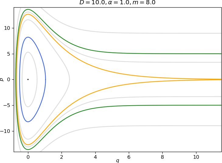
Trajectories with energies larger than $D$ have unbounded motion in $q$. Trajectories having energies $h$ satisfying $0< h < D$ correspond to periodic motions. The level sets of these periodic orbits are given by:

\begin{equation} h= \frac{p^2}{2m} + D \left( 1-e^{-\alpha q} \right)^2, \quad 0< h < D, \label{eq:tp1} \end{equation}

and surround the stable equilibrium point $(q, p) = (0, 0)$ as shown in figure fig:1. The periodic orbits intersect the $q$ axis at two distinct points, $q_+ > 0$ and $q_- <0$, which are referred to as turning points. These turning points are computed as follows.

Rewriting \eqref{eq:tp1} gives:

\begin{equation} \frac{p^2}{2m} = h- D \left( 1-e^{-\alpha q} \right)^2. \label{eq:tp2} \end{equation}

The turning points are obtained from \eqref{eq:tp2} by setting $p=0$:

\begin{equation} h=D \left( 1-e^{-\alpha q} \right)^2 \label{eq:tp3} \end{equation}

Note that we have:

\begin{equation} 0 \le \sqrt{\frac{h}{D}} \le 1, \label{eq:tp4} \end{equation}

from which we obtain the following relations:

\begin{eqnarray} && 1 \le 1 + \sqrt{\frac{h}{D}} \le 2, \label{eq:tp5} \\ && 0 \le 1 - \sqrt{\frac{h}{D}} \le 1, \label{eq:tp6} \end{eqnarray}

Taking the positive root of \eqref{eq:tp3} gives:

\begin{equation} 1-e^{-\alpha q} = \sqrt{\frac{h}{D}}. \label{eq:tp7} \end{equation}

from which we obtain the positive turning point:

\begin{equation} q_+ = - \frac{1}{\alpha} \log \left(1- \sqrt{\frac{h}{D}} \right) > 0. \label{eq:tppos} \end{equation}

Taking the negative root of \eqref{eq:tp3} gives:

\begin{equation} 1-e^{-\alpha q} = -\sqrt{\frac{h}{D}}, \label{eq:tp8} \end{equation}

from which we obtain the negative turning point:

\begin{equation} q_- = - \frac{1}{\alpha} \log \left(1 + \sqrt{\frac{h}{D}} \right) < 0. \label{eq:tpneg} \end{equation}

The level curve with energy equal to the dissociation energy $h=D$ has the form:

\begin{equation} D= \frac{p^2}{2m} + D \left( 1-e^{-\alpha q} \right)^2, \label{eq:homo1} \end{equation}

and is a separatrix connecting the (parabolic) saddle point. In the terminology of Hamiltonian dynamics it is a homoclinic orbit. It separates bounded from unbounded motion as illustrated in figure fig:1.

---

Calculation of the Period of a Periodic Orbit

In this section we calculate the period of the periodic orbits. From \eqref{eq:hameq} we have $\dot{q} = \frac{p}{m}$. Using this expression, and the expression for the level set of the Hamiltonian defining a periodic orbit given in \eqref{eq:tp1}, we have

\begin{equation} \frac{dq}{dt} = \pm \sqrt{\frac{2}{m}} \sqrt{h-D \left( 1-e^{-\alpha q} \right)^2}, \label{eq:po1} \end{equation}

or

\begin{equation} \frac{dq}{ \sqrt{h-D \left( 1-e^{-\alpha q} \right)^2}} = \pm \sqrt{\frac{2}{m}} dt. \label{eq:po2} \end{equation}

We denote the period of a periodic orbit corresponding to the level set with energy value $h$ by $T(h)$. We can obtain the period by integrating $dt$ around this level set. Using \eqref{eq:po2}, this becomes:

\begin{eqnarray} T(h) & = & \sqrt{\frac{m}{2}} \int_{q_+}^{q_-} \frac{dq}{ \sqrt{h-D \left( 1-e^{-\alpha q} \right)^2}} - \sqrt{\frac{m}{2}} \int_{q_-}^{q_+} \frac{dq}{ \sqrt{h-D \left( 1-e^{-\alpha q} \right)^2}}. \nonumber \\ & = & \sqrt{2m} \int_{q_+}^{q_-} \frac{dq}{ \sqrt{h-D \left( 1-e^{-\alpha q} \right)^2}}. \label{eq:po3} \end{eqnarray}

Computation of this integral is facilitated by the substitution:

\begin{equation} u = e^{-\alpha q}. \label{eq:subs} \end{equation}

After computing the integral using integral 2.266 in (missing reference) we obtain:

\begin{equation} T(h) = \frac{\pi \sqrt{2m}}{\alpha \sqrt{D-h}} \label{eq:period} \end{equation}

There are two limits in which this expression can be checked with respect to previously obtained results. First, we note that for $h=D$ (i.e. the energy of the homoclinic orbit, or ''separatrix'') $T(D) = \infty$, which is what we expect for the ''period'' of a separatrix.

Second, we consider $h=0$, which is the energy of the elliptic equilibrium point. In this case we have $T(0) = \frac{\pi \sqrt{2m}}{\alpha \sqrt{D}}$, which is $2 \pi$ divided by the imaginary part of the magnitude of eigenvalue of the Jacobian evaluated at the stable equilibrium point, as we expect.

Calculation of position and momentum: $q(t)$ and $p(t)$, $0 < h < D$

In this section we derive an expression for $q(t)$. Differentiating the expression for $q(t)$ will give the expression for $p(t)$ through the relation $\dot{q} = \frac{p}{m}$. Using \eqref{eq:po2}, we have

\begin{equation} \int_{q_+}^q \frac{dq'}{ \sqrt{h-D \left( 1-e^{-\alpha q'} \right)^2}} = \sqrt{\frac{2}{m}} t. \label{eq:traj1} \end{equation}

Choosing the lower limit if the integral to be $q_+$ is arbitrary, but it is equivalent to the choice of an initial condition. After computing this integral, we obtain:

\begin{equation} q(t) = \frac{1}{\alpha} \log{\frac{\sqrt{Dh} \cos \left(\sqrt{\frac{2(D-h)}{m}} \, \alpha t \right) + D}{D-h}}. \label{eq:q(t)} \end{equation}

It is straightforward to check that the period of \eqref{eq:q(t)} is \eqref{eq:period}.

Calculation of the Homoclinic Orbit: $q_0(t)$ and $p_0(t)$, $0 < h < D$

As noted earlier, the homoclinic orbit, corresponding to $h=D$, is given by the level set \eqref{eq:homo1}. Hence, the integral expression for the homoclinic orbits is obtained from \eqref{eq:po2} by setting $h=D$. Computing the integral gives:

\begin{equation} q_0(t) = \frac{1}{\alpha} \log{\frac{1 + \frac{2D}{m} \alpha^2 t^2}{2}}. \label{eq:qhom} \end{equation}

It is a simple matter to check that $\lim_{t \rightarrow \pm \infty} q(t) = \infty$. Subsequently we obtain $p_0(t)$ from $\dot{q}=\frac{p}{m}$ as

\begin{equation} p_0(t) = \frac{4mD\alpha t}{2D\alpha^2 t^2+m}. \label{eq:phom} \end{equation}

Calculation of the Action-Angle coordinates: $I$ and $\theta(t)$, $0 < h < D$

In this section we compute the action-angle representation of the orbits in the bounded region following [2], [3], [4].

We consider a level set defined by the Hamiltonian \eqref{eq:levelset}, for $0 < h < D$. i.e. we consider a periodic orbit with period $T(h)$. Choosing an arbitrary reference point on the periodic orbit, the angular displacement of a trajectory starting from this reference position after time $t$ is given by:

\begin{equation} \theta = \frac{2 \pi}{T(h)} \int{0}^{t}dt' = \frac{2 \pi}{T(h)} \sqrt{\frac{m}{2}} \int_{q_+}^q \frac{dq'}{ \sqrt{h-D \left( 1-e^{-\alpha q'} \right)^2}}. \label{eq:angle1} \end{equation}

Using the substitution \eqref{eq:subs} and integral 2.266 in (missing reference), we have:

\begin{equation} \theta = \frac{\pi}{T(h)\alpha} \sqrt{\frac{2m}{D-h}} \left(\frac{3\pi}{2} - \sin^{-1}\frac{(h-D)e^{\alpha q}+D}{\sqrt{Dh}} \right). \label{eq:angle2} \end{equation}

The action associated with this periodic orbit is the area that it encloses (in phase space) divided by $2 \pi$:

\begin{equation} I = \frac{1}{2 \pi} \oint_{H=h} p dq. \label{eq:action1} \end{equation}

Recalling \eqref{eq:po2}

\begin{equation} dq = \pm \sqrt{\frac{2}{m}}\sqrt{h-D \left( 1-e^{-\alpha q'} \right)^2} \, dt, \label{eq:action2} \end{equation}

we obtain:

\begin{equation} pdq = m \dot{q} dq = \pm \sqrt{2m}\sqrt{h-D \left( 1-e^{-\alpha q'} \right)^2} \, \dot{q}dt, \label{eq:action3} \end{equation}

and therefore

\begin{equation} I = \frac{\sqrt{2m}}{\pi} \int_{q_+}^{q_-}\sqrt{h-D \left( 1-e^{-\alpha q'} \right)^2} \, dq'. \label{eq:action4} \end{equation}

Using the substitution \eqref{eq:subs} and integral 2.267 in (missing reference), we have:

\begin{equation} I = \frac{\sqrt{2m}}{\alpha} \left(\sqrt{D}-\sqrt{D-h}\right). %checked \label{eq:action5} \end{equation}

Expressions for $q(t)$ and $p(t)$, $0 < D < h$

Increasing the total energy $h$ to the value of $D$ and beyond results in unbounded motion. Trajectories retain the turning point $q_-$, while $q_+$ becomes infinite. The expression for $q_-$ is identical to low energies and is obtained from \eqref{eq:ham} by setting $p=0$ and solving for $q$. Recall from \eqref{eq:tpneg} that $q_- = - \frac{1}{\alpha} \log \left(1 + \sqrt{\frac{h}{D}} \right)$.

For unbounded trajectories it is not possible to define a (finite) period, but we can obtain an expression for $t$ as a function of position. It can be derived by integrating \eqref{eq:po2} from $q_-$ to an arbitrary position $q$ by using the substitution \eqref{eq:subs} as follows:

\begin{eqnarray} t(q) & = & \sqrt{\frac{m}{2}} \int_{q}^{q_-} \frac{dq'}{ \sqrt{h-D \left( 1-e^{-\alpha q'} \right)^2}}= -\frac{1}{\alpha}\sqrt{\frac{m}{2}} \int_{e^{-\alpha q}}^{1+\sqrt{\frac{h}{D}}} \frac{du}{u \sqrt{h-D \left( 1-u \right)^2}},\nonumber \\ & = & \frac{1}{\alpha}\sqrt{\frac{m}{2(h-D)}} \log{\left(\frac{h-D+De^{-\alpha q}+\sqrt{(h-D)(h-D(1-e^{-\alpha q})^2)}}{\sqrt{hD}e^{-\alpha q}}\right)}. %checked \label{eq:tinf} \end{eqnarray}

We obtain an explicit solution $q=q(t)$ by inverting \eqref{eq:tinf}.

\begin{equation} q(t) = \frac{1}{\alpha} \log{ \frac{\sqrt{hD}e^{2\beta t} -2De^{\beta t} + \sqrt{hD}}{2(h-D)e^{\beta t}} }, %checked \label{eq:qinf} \end{equation}

where $\beta=\alpha\sqrt{\frac{2(h-D)}{m}}$. Differentiating \eqref{eq:qinf} and using the relation $\dot{q} = \frac{p}{m}$ yields the expression of $p(t)$.

Implications for reaction dynamics

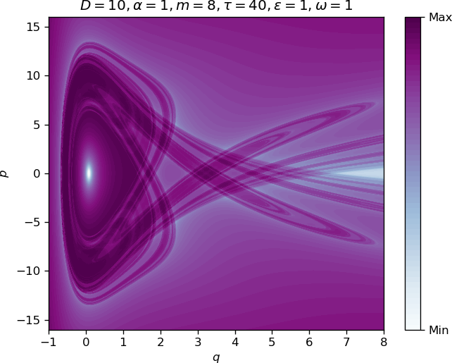
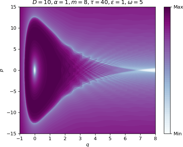
Once explicit solutions are known, it is insightful to consider how they change when the vector field is changed, slightly. This is considered in the field of perturbation theory. The subharmonic and homoclinic Melnikov [3] are examples of global perturbation methods that consider the effect of perturbations on the entire unperturbed integrable system, such as the Morse oscillator that we have considered. The type of perturbation that we will consider is a time periodic excitation of the Morse oscillator. The subharmonic and homoclinic Melnikov methods for this system have been previously considered in (missing reference), however, with respect to chaotic dynamics, important technical details for this periodically perturbed Morse oscillator were not considered. We will describe these in detail here, as well as consider the nature of the effect of the parameters of the Morse potential, and the periodic excitation, on chaotic dynamics.

The homoclinic Melnikov function is a well-known and popular method for proving the existence of chaos, in the sense of Smale horseshoes, in time periodically perturbed one degree-of-freedom Hamiltonian systems. The method allows one to prove the existence of transverse homoclinic periodic orbits to a hyperbolic periodic orbit. Such orbits admit a Smale horseshoe construction. There are two issues with the application of the standard homoclinic Melnikov function to the time periodically perturbed Morse oscillator, and both issues arise from the fact that the saddle point at infinity is parabolic, not hyperbolic. One issue is the fact that the standard derivation of the homoclinic Melnikov function uses hyperbolicity of the fixed point to show that certain terms in the Melnikov function vanish. The other issue involves the construction of the Smale horseshoe map for orbits homoclinic to a parabolic point. Both issue are considered for the perturbed Morse oscillator in (missing reference) where it is shown that the growth and decay properties for the parabolic point in the Morse oscillator are sufficient for the standard Melnikov function to be valid as well as the Smale horseshoe map construction to be valid. Hence, the ''Melnikov approach'' is sufficient for determining the existence of chaos for the time-periodically perturbed Morse oscillator.

We consider the following time-periodic perturbation of the Morse oscillator:

\begin{eqnarray} \dot{q} = \frac{\partial H}{\partial p} & = & \frac{p}{m}, \nonumber \\ \dot{p} = - \frac{\partial H}{\partial q} & = & -2D \alpha \left(e^{-\alpha q} - e^{-2\alpha q} \right) +\varepsilon \cos{\omega t}, \label{eq:perteq} \end{eqnarray}

where $\varepsilon>0$ is the magnitude of the perturbation and $\omega>0$ the frequency of the perturbation. The unperturbed system \eqref{eq:hameq} is obtained by setting $\varepsilon=0$. We formulate the homoclinic Melnikov function using expressions \eqref{eq:qhom}, \eqref{eq:phom} for $q_0(t)$, $p_0(t)$, the homoclinic orbit of the equilibrium point $(q,p)=(\infty,0)$, as follows:

\begin{equation} M(t_0,\phi_0)=\int\limits_{-\infty}^{\infty} DH(q_0(t),p_0(t))\cdot(0, \varepsilon \cos(\omega t+\omega t_0+\phi_0)) dt, \label{eq:Melnikovdef} \end{equation}

where $DH$ is the gradient of the unperturbed Hamiltonian \eqref{eq:ham}, $t_0$ defines the point $(q_0(t_0),p_0(t_0))$ at which the Melnikov funtion $M$ is evaluated and $\phi_0$ is the time at which $M$ is evaluated. We solve \eqref{eq:Melnikovdef} using integral 3.723 in (missing reference).

\begin{eqnarray} M(t_0,\phi_0)&=&\varepsilon \int\limits_{-\infty}^{\infty} \frac{\partial H}{\partial p}(q_0(t),p_0(t)) \cos(\omega t+\omega t_0+\phi_0) dt,\nonumber \\ &=& \varepsilon \int\limits_{-\infty}^{\infty} \frac{p_0(t)}{m} \left( \cos(\omega t)\cos(\omega t_0+\phi_0)-\sin(\omega t)\sin(\omega t_0+\phi_0) \right) dt, \nonumber\\ &=& -\varepsilon \frac{2m}{\alpha} \sin(\omega t_0+\phi_0) \int\limits_{-\infty}^{\infty} \frac{t}{t^2+\frac{m}{2D\alpha^2}} \sin(\omega t) dt, \nonumber\\ &=& -\varepsilon \frac{2m}{\alpha} \sin(\omega t_0+\phi_0) e^{-\omega\sqrt{\frac{m}{2D\alpha^2}}}. \label{eq:Melnikovsol} \end{eqnarray}

Clearly, this function has ''simple zeros'' indicating the existence of homoclinic orbits, and the associated Smale horseshoe type chaos.

The magnitude of the Melnikov function is a measure of the intensity of the chaos. Since the exponent in the exponential term is negative, $$e^{-\omega\sqrt{\frac{m}{2D\alpha^2}}}\leq 1.$$ The exponent is decreased by decreasing $\omega$ and $m$, and increasing $\alpha$ and $D$. Note that $M$ is monotonically increasing in dissociation energy $D$, yet the homoclinic orbit ceases to exist for $D=\infty$.

The dominant term in the Melnikov functions is $$\frac{2m}{\alpha}.$$ To reach the highest intensity of chaos in the system, $m$ has to be large and $\alpha$ small, whereby the mitigating effect of the exponential term can be countered by choosing $D>\frac{m}{\alpha^2}$. Then for any $\omega$ we can find $(t_0,\phi_0)$, such that $\sin(\omega t_0+\phi_0)=1$ and

\begin{equation} |M(t_0,\phi_0)|=\varepsilon \frac{2m}{\alpha} e^{-\omega\sqrt{\frac{m}{2D\alpha^2}}} > \varepsilon \frac{2m}{\alpha}e^{-\frac{\omega}{\sqrt{2}}}. \label{eq:Melnikovmag} \end{equation}

In figure fig:2 we show a comparison of different intensities of chaos using Lagrangian descriptors, a method introduced by (missing reference) and proven to display invariant manifolds in two dimensional area-preserving maps by (missing reference).

---

An animation showing the effect of varying $\omega$ can be found here

References

1. P. M. Morse, “Diatomic molecules according to the wave mechanics. II. Vibrational levels,” Physical Review, vol. 34, no. 1, p. 57, 1929.
2. V. K. Melnikov, “VK Melnikov, Trans. Moscow Math. Soc. 12, 1 (1963).,” Trans. Moscow Math. Soc., vol. 12, p. 1, 1963.
3. S. Wiggins, “Introduction to applied nonlinear dynamical systems and chaos,” 1990.
4. I. Mezić and S. Wiggins, “On the integrability and perturbation of three-dimensional fluid flows with symmetry,” Journal of Nonlinear Science, vol. 4, no. 1, pp. 157–194, 1994.
5. H. S. Dumas, The KAM Story: A Friendly Introduction to the Content, History, and Significance of Classical Kolmogorovâ Arnoldâ Moser Theory. World Scientific Publishing Company, 2014.
6. A. D. Stone, “Einstein’s unknown insight and the problem of quantizing chaos,” Physics Today, vol. 58, no. 8, p. 37, 2005.
7. J. B. Keller, “Corrected Bohr-Sommerfeld quantum conditions for nonseparable systems,” Annals of Physics, vol. 4, no. 2, pp. 180–188, 1958.
8. J. B. Keller and S. I. Rubinow, “Asymptotic solution of eigenvalue problems,” Annals of Physics, vol. 9, no. 1, pp. 24–75, 1960.
9. J. B. Keller, “Semiclassical mechanics,” Siam Review, vol. 27, no. 4, pp. 485–504, 1985.