
Introduction
Molecular reaction dynamics is concerned with the breaking and forming of bonds between the atoms that make up a molecule. The description of such mechanisms requires analyzing how the bonds change in time, that is, it is a dynamical mechanism requiring a phase space description. The phase space will have coordinates that correspond to the bond configurations with a corresponding canonical momentum for each bond configuration coordinate. Thus, the dynamics of chemical bonds can be formulated in the language of Hamiltonian dynamics and its resulting phase space geometry. In recent years there has been significant developments in the mathematical description and analysis of chemical reaction dynamics in phase space [1], [2], [3].
Our objective is to describe the change in a bond that signals the occurrence of a chemical reaction in terms of a unique characteristic of a trajectory of Hamilton's equations. This characteristic requires an understanding of the geometry of the phase space of the molecule in a way that enables us to divide an appropriate volume of phase space into a region corresponding to ''reactants'' and a region corresponding to ''products''. The passage from reactants to products, that is ''reaction'', occurs when a trajectory crosses the ''dividing surface'' (DS) between the reactants and products. In this framework for understanding chemical reactions, the flux through such a dividing surface would be related to the reaction rate, and therefore the construction of a DS between such regions is of interest in reaction dynamics. The description of the regions of reactants and products can often be inferred from the nature of the development of the coordinates used in the mathematical model of the chemical reaction. Once the model is developed, the DS must be constructed in the context of this model. In relating the flux through the DS to a reaction rate it is desirable that trajectories crossing the DS from the reactant side proceed to the product side before possibly recrossing the DS back to the reactant region. Thus, we require the DS to have the ''no-recrossing'' property [4], [5]. Since Hamiltonian dynamics conserves energy, the trajectories evolve on the energy surface, which is of codimension one in phase space. The DS is required to be codimension one in the energy surface. Hence, we require a DS between reactants and products to be codimension one in the energy surface and to have the no-recrossing property. We note that Wigner had already described these properties for a DS in phase space much earlier [6], [7], and a review of classical and quantum versions of DS constructed in phase space can be found in [8].
The construction of a DS separating the phase space into two parts, reactants and products, has been a focus from the dynamical systems point of view in recent years. However, the lack of a firm theoretical basis for the construction of such surfaces for molecular systems with three and more degree-of-freedom (DoF) has until recently been a major obstacle in the development of the theory. In phase space, that is for nonzero momentum, the role of the saddle point is played by an invariant manifold of saddle stability type, the normally hyperbolic invariant manifold (NHIM) (see sec:HSN_2DOF) [9], [10], [11]. In order to fully appreciate the NHIM and its role in reaction rate theory, it is useful to begin with a precursor concept -- the periodic orbit dividing surface or PODS. For systems with two DoF described by a natural Hamiltonian, kinetic plus potential energy, the problem of constructing the DS in phase space was solved during the 1970s by McLafferty, Pechukas and Pollak [12], [13], [14], [15]. They demonstrated that the DS at a specific energy is related to an invariant phase space structure, an unstable periodic orbit (UPO). The UPO defines (it is the boundary of) the bottleneck in phase space through which the reaction occurs and the DS which intersects trajectories evolving from reactants to products can be shown to have the geometry of a hemisphere in phase space whose boundary is the unstable PO [16], [5]. The same construction can be carried out for a DS intersecting trajectories crossing from products to reactants and these two hemispheres form a sphere for which the UPO is the equator. Generalisation of this construction of DS to high dimensional systems has been a central question in reaction dynamics and has only received a satisfactory answer in recent years [16], [2]. The key difficulty concerns the high dimensional analogue of the unstable PO used in the two DoF system for the construction of the DS. This difficulty is resolved by considering the NHIM, which has the appropriate dimensionality for anchoring the dividing surface in phase space.
Results from dynamical systems theory show that transport in phase space is controlled by high dimensional manifolds, NHIMs, which are the natural generalisation of the UPO of the two DoF case [10]. Normal hyperbolicity of these invariant manifolds means that their stability, in a precise sense, is of saddle type in the transverse direction, which implies that they possess stable and unstable invariant manifolds that are impenetrable barriers and mediate transport in phase space. These invariant manifolds of the NHIM are structurally stable, that is, stable under perturbation [11].
In this chapter we describe the influence of Hamiltonian saddle-node bifurcations on the high-dimensional phase space structures that mediate transport and characterize reaction dynamics [17]. We do so by identifying the relevant invariant manifolds, NHIMs and their stable and unstable manifolds, using the method of Lagrangian descriptors (LDs). In a general context, a saddle-node bifurcation takes place when a saddle and an elliptic equilibrium point of a dynamical system 'collide' as the value of a physical parameter is varied. This phenomenon occurs naturally in a Chemistry setup as a consequence of lowering the energy barrier height associated to a saddle point of a given potential energy surface (PES), which results in the connection of the potential well region on one side of the saddle to a escape channel. Therefore, this mechanism facilitates that trajectories cross the phase space bottleneck in the neighborhood of the index-1 saddle, and hence has a great influence on reaction dynamics. The drastic changes produced in the geometry of the phase space structures can then be used to account for corrections to Kramers' reaction rate as the barrier height decreases [18], providing a significant step for the experimental study of single bond dynamics of molecules and the control of micro- and nano-electromechanical devices [18], [19], [20], [21]. A nice example regarding the influence of Hamiltonian saddle-node bifurcations on isomerization dynamics can be found in that of the LiCN/LiNC molecule [22], [23], [24]. Other applications include the study of ionization and dissociation rates in atomic systems [25], [26], [27], [28], [29], [30], [31], [32].
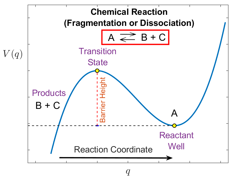
In the framework of chemical reaction dynamics, saddle-node bifurcations occur in problems that address the escape from a potential well by crossing an energy barrier and the influence that the barrier height has on the reactive flux. These situations can be identified for instance with dissociation or fragmentation reactions, where a chemical transformation takes place if the bond of a molecule A breaks up, giving rise to two products B and C. In this situation, the equilibrium conformation of the given molecule A is represented by a potential well in a PES, and dissociation into B and C can take place if the system has sufficient energy to cross the potential barrier that separates bounded (vibration) from unbounded (bond breakup) motion. This phenomenon can be modeled for instance by means of a cubic potential energy function as illustrated in Fig. fig:1, which will be our building block to construct the normal form Hamiltonian that describes saddle-node bifurcations in phase space. Our goal is to determine the geometrical phase space structures that ''divide'' reactants from products, and identify dynamically distinct phase space regions corresponding to reactive and non-reactive initial conditions for the dynamical system.
In this section we introduce the normal form Hamiltonian that determines saddle-node bifurcations for systems with two DoF. The natural extension of our previous one DoF model is to add another DoF called x, in the form of a harmonic oscillator with frequency ω>0 and mass m=1. This extra DoF plays the role of a bath mode in the terminology of chemical reaction dynamics, and we suppose a quadratic coupling with the reactive DoF q. Under these assumptions, the Hamiltonian becomes:
H(q,x,p,px)=12(p2+p2x)−√μq2+α3q3+ω22x2+ε2(x−q)2,where ε⩾ is the strength of the coupling between the reaction and the bath mode, and the kinetic (T) and potential (V) energies are given by:
\begin{equation} T(p,p_x) = \frac{1}{2}\left(p^2 + p_x^2\right) \quad,\quad V(q,x) = - \sqrt{\mu} \, q^2 + \frac{\alpha}{3} \,q^3 + \dfrac{\omega^2}{2} x^2 + \dfrac{\varepsilon}{2} \left(x-q\right)^2 \label{eq:pes_2dof} \end{equation}For this Hamiltonian, the equations of motion have the form:
\begin{equation} \begin{cases} \dot{q} = \dfrac{\partial H}{\partial p} = p \\[.4cm] \dot{x} = \dfrac{\partial H}{\partial p_x} = p_x \\[.4cm] \dot{p} = -\dfrac{\partial H}{\partial q} = 2\sqrt{\mu} \, q - \alpha \, q^2 + \varepsilon (x - q) \\[.4cm] \dot{p}_x = -\dfrac{\partial H}{\partial x} = -\omega^2 x + \varepsilon (q-x) \end{cases} \label{eq:hameq_2dof} \end{equation}The phase space for this dynamical system is four dimensional, and due to energy coservation, trajectories evolve on a three dimensional energy hypersurface.
For the Hamiltonian system that we are analyzing, we would like to point out that there exists a simple and interesting mathematical connection between the coupling parameter, the eigenfrequencies at the barrier which determine the local dynamics in the phase space bottleneck region and the geometry of the PES, described by means of the Gaussian curvature. For a given surface V(x,y), the Gaussian curvature can be calculated from the following formula [33] :
\begin{equation} \mathcal{K} = \dfrac{\det \left(\mathcal{H}_V\right)}{\left(1 + \| \nabla V \|^2\right)^2} \end{equation}where \mathcal{H}_V denotes the Hessian matrix associated to the PES. It is straightforward to show then that the coupling strength linearly determines the Gaussian curvature at the minimum of the well and the barrier of the PES:
\begin{equation} \mathcal{K}_{\text{well}} = \left(\omega^2 - 2\sqrt{\mu}\right) \left(\varepsilon_c - \varepsilon\right) \quad , \quad \mathcal{K}_{\text{barrier}} = -\mathcal{K}_{\text{well}} \end{equation}and that the proportionality constant depends only on the difference of the squares of the eigenfrequencies of the uncoupled system at the barrier region. This means that the local geometry of the bottleneck can be controlled by these parameters.
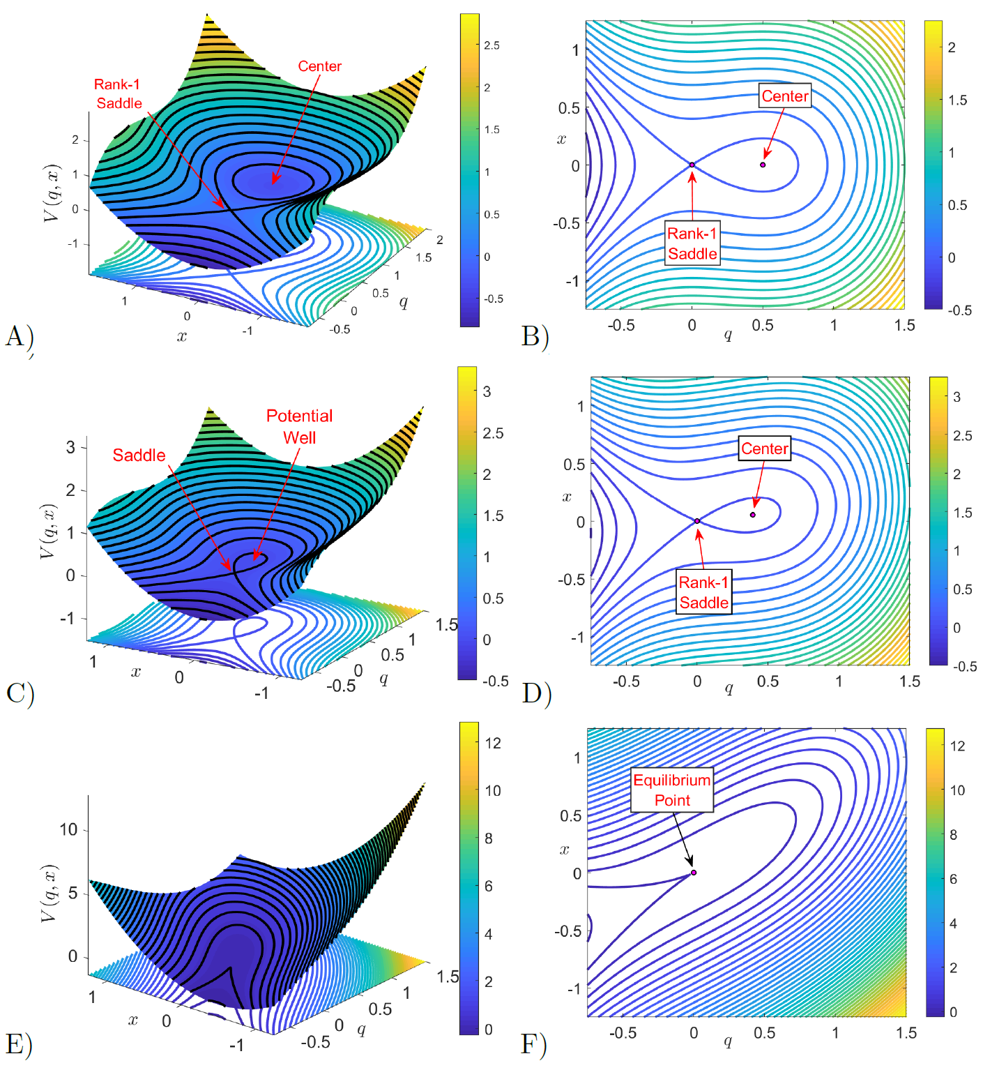
We illustrate in Fig. fig:2 how the geometry of the PES changes as the coupling strength \varepsilon is varied. For this visualization, we have used the following values of the model parameters \mu = 0.25, \alpha = 2, and \omega = 1.25. The reason for doing so is that they satisfy the condition \omega^2 > 2\sqrt{\mu} and consequently a critical value of the perturbation parameter exists, given by \varepsilon_c = 25/9, at which the two equilibrium points 'collide' at the origin resulting in a saddle-node bifurcation. The dynamics after this collision is beyond the scope of this study and therefore we will only focus on the description of the system dynamics for different values of the coupling strength \varepsilon < \varepsilon_c. Observe in Fig. fig:2 A) and B) that the location of the well lies on the q-axis when the DoF are uncoupled (\varepsilon = 0). As \varepsilon is increased, Fig. fig:2 C) and D) show that its effect is to tilt the PES with respect to the configuration space plane, and the position of the potential well moves off the q-axis towards the origin. Finally, the situation for which the coupling strength reaches the critical value \varepsilon_c is shown in Fig. fig:2 E) and F) for which the collision has happened and there is only one critical point of the potential at the origin.
It is straightforward to check that the equilibrium points for this system are located at:
\begin{equation} \mathbf{x}_1^e = (0,0,0,0) \quad,\quad \mathbf{x}_2^e = \frac{2\sqrt{\mu} \, \omega^2 + \left(2\sqrt{\mu}-\omega^2\right)\varepsilon}{\alpha \, (\omega^2 + \varepsilon)} \left(1,\frac{\varepsilon}{\omega^2 + \varepsilon},0,0\right) \label{eq:cfSp_eqCoords} \end{equation}Notice that there exists a critical value for the coupling strength:
\begin{equation} \varepsilon_c = \dfrac{2\sqrt{\mu} \, \omega^2}{\omega^2 - 2\sqrt{\mu}} \;, \label{eq:critepsi} \end{equation}for which the Hamiltonian in Eq. \eqref{eq:hameq_2dof} has only one equilibrium point at the origin, and interestingly, a saddle-node bifurcation takes place in phase space when \varepsilon = \varepsilon_c. We will analyze later the influence of the perturbation strength \varepsilon on the geometry of the phase space structures. Observe that this critical value is independent of the nonlinearity strength parameter \alpha and requires \omega^2 > 2\sqrt{\mu} to be satisfied, since the coupling strength \varepsilon is a non-negative parameter. Moreover, the critical coupling is characterized by a functional relationship between the squares of the eigenfrequencies of the reactive and bath DoF of the uncoupled system (\varepsilon = 0). Physically, the interpretation of this condition is that the bath mode has more influence on the dynamics of the system than that of the reactive DoF, which describes the behavior in the vicinity of the barrier. In the limiting case where \omega^2 = 2\sqrt{\mu}, the configuration space coordinates of the equilibrium point \mathbf{x}_2^e corresponding to the potential well are:
\begin{equation} q_e = \frac{4\mu}{\alpha(2\sqrt{\mu} + \varepsilon)} \quad,\quad x_e = \frac{4\mu \, \varepsilon}{\alpha(2\sqrt{\mu} + \varepsilon)^2} \end{equation}showing that this point approaches the origin as \varepsilon \to \infty, and therefore no bifurcation occurs in this situation. Finally, for the case \omega^2 < 2\sqrt{\mu} we have seen that there is no bifurcation as \varepsilon is varied. In fact, if \varepsilon \to \infty the potential well will approach the limit point in configuration space:
\begin{equation} q_e = x_e = \frac{2\sqrt{\mu} - \omega^2}{\alpha} > 0 \end{equation}At this point, we carry out a linear stability analysis to show that the equilibrium point at the origin is an index-1 saddle of the PES. This analysis will be useful for computing the unstable periodic orbit (UPO), or normally hyperbolic invariant manifold (NHIM), associated to the index-1 saddle. Also, it will allow us to determine the NHIM's invariant stable and unstable manifolds that act as codimension one impenetrable barriers on the constant energy hypersurface. The global geometry of these invariant manifolds is paramount for quantifying the reaction rate across the phase space bottleneck in the neighborhood of the index-1 saddle. The Jacobian matrix for the Hamiltonian system in Eq. \eqref{eq:hameq_2dof} is given by:
\begin{equation} J(q,x,p,p_x) = \begin{pmatrix} 0 & 0 & 1 & 0 \\[.1cm] 0 & 0 & 0 & 1 \\[.1cm] 2\sqrt{\mu} - 2\alpha q - \varepsilon & \varepsilon & 0 & 0 \\[.1cm] \varepsilon & -\omega^2 - \varepsilon & 0 & 0 \end{pmatrix} \end{equation}The stability of \mathbf{x}_1^e = (0,0,0,0) is given by the eigenvalues of the Jacobian:
\begin{equation} J(\mathbf{x}_1^e) = \begin{pmatrix} 0 & 0 & 1 & 0 \\[.1cm] 0 & 0 & 0 & 1 \\[.1cm] 2\sqrt{\mu} - \varepsilon & \varepsilon & 0 & 0 \\[.1cm] \varepsilon & -\omega^2 - \varepsilon & 0 & 0 \end{pmatrix} \label{eq:jacobian_2dof} \end{equation}If the system is decoupled, i.e. \varepsilon = 0, the eigenvalues are given by \pm \lambda_0 and \pm \omega_0 \, i, where:
\begin{equation} \lambda_0 = \sqrt[4]{4\mu} \;,\quad \omega_0 = \omega \end{equation}Therefore, the origin is an index-1 saddle equilibrium point, since the linearized system has exactly one pair of real eigenvalues \pm \lambda_0 and the saddle plane is spanned by their eigenvectors. We know from the Moser's generalization of the Lyapunov Subcenter Theorem [11], [34] that when the energy of the system is above that of the index-1 saddle, there is a two dimensional plane spanned by the eigenvectors of \pm \omega_0 \, i, known as the center invariant manifold. This invariant manifold with normal hyperbolicity is known as a NHIM and in the context of Hamiltonian systems with 2 DoF is an UPO and has the topology of a circle S^1. As the energy of the system is increased above the energy of the index-1 saddle at the origin, a bottleneck structure opens in phase space connecting dynamically different regions and allowing trajectories to move between them. This phenomenon results in a phase space transport mechanism. This framework of understanding chemical reactions is realized by computing the stable and unstable manifolds associated with the unstable periodic orbit. These invariant manifolds have cylindrical geometry, that is \mathbb{R} \times S^1, and their global behavior is referred to as tube dynamics. The cylindrical manifolds are codimension one on the constant three-dimensional energy hypersurface and therefore, act as impenetrable barriers separating reactive and non-reactive trajectories in the phase space. Thus, they determine the initial conditions that will pass through the bottleneck in some future time (or had passed through it in the past) during their evolution~[35]. The UPO provides us with the scaffolding to construct the dividing surface that separates the trapped motion in the well region of the PES and the escape to infinity of particle trajectories through the phase space bottleneck.
We look now at the linear stability of the coupled system, that is \varepsilon \neq 0. In this case, the reaction and bath DoF are coupled and we expect chaotic trajectories to appear, having a significant influence on the reaction rate. However, the geometry of the NHIM and its invariant manifolds still governs this reaction mechanism. A simple analysis reveals that the square of the eigenvalues of the Jacobian matrix at the origin are given by:
\begin{equation} \xi =\dfrac{\lambda_0^2 - \omega_0^2}{2} - \varepsilon \pm \sqrt{\left(\dfrac{\lambda_0^2 + \omega_0^2}{2}\right)^2 + \varepsilon^2} \;\;. \label{eq:eigham2dof} \end{equation}as a function of the coupling strength \varepsilon and the squares of the eigenvalues of the uncoupled system \lambda_0^2 and \omega_0^2. Notice that when the condition \omega_0^2 \leq \lambda_0^2 holds, the two possible values of \xi have opposite signs for all \varepsilon > 0. Moreover, under the assumption \omega_0^2 > \lambda_0^2, the two values of \xi have opposite sign whenever 0 < \varepsilon < \varepsilon_c is satisfied, where the critical coupling strength \varepsilon_c is given by Eq. \eqref{eq:critepsi}. If we denote \xi_{1,\varepsilon} and \xi_{2,\varepsilon} as the positive and negative roots respectively in Eq. \eqref{eq:eigham2dof}, then the eigenvalues of the Jacobian matrix are \pm \lambda_\varepsilon and \pm \omega_\varepsilon i where:
\begin{equation} \lambda_\varepsilon = \sqrt{\xi_{1,\varepsilon}} \quad,\quad \omega_\varepsilon = \sqrt{|\xi_{2,\varepsilon}|} \;. \label{eq:eigenvalues_2dof} \end{equation}This argument shows that the equilibrium point at the origin is still an index-1 saddle for the coupled system under the conditions discussed above. In particular, when the coupling between the reaction and the bath DoF is weak, that is \varepsilon \ll 1, we have:
\begin{equation} \lambda_\varepsilon \approx \sqrt{\lambda_0^2 - \varepsilon} \quad,\quad \omega_\varepsilon \approx \sqrt{\omega_0^2 + \varepsilon} \;, \end{equation}which confirms that the index-1 saddle structure of the equilibrium point at the origin persists under small perturbations. To finish the linear stability analysis of the equilibrium point at the origin, we compute the eigenvectors. Those associated with the real eigenvalues \beta = \pm \lambda_{\varepsilon} correspond to the tangent directions of the unstable and stable manifolds, respectively, of the NHIM at the index-1 saddle, are given by:
\begin{equation} \mathbf{u}_{\pm} = \left(1,\frac{\varepsilon}{\varepsilon + \left(\lambda^2_\varepsilon + \omega^2_0\right)},\pm\lambda_{\varepsilon},\pm\frac{\lambda_{\varepsilon} \, \varepsilon}{\varepsilon + \left(\lambda^2_\varepsilon + \omega^2_0\right)}\right) \;. \label{eq:saddle_eigenv} \end{equation}The eigenvectors associated with the complex eigenvalues \beta = \pm \omega_\varepsilon i span the center subspace of the NHIM at the index-1 saddle have the form:
\begin{equation} \mathbf{w}_{\pm} = \left(\frac{\varepsilon}{\varepsilon - \left(\lambda^2_0 + \omega^2_\varepsilon\right)},1,\pm\frac{\omega_{\varepsilon} \, \varepsilon}{\varepsilon - \left(\lambda^2_0 + \omega^2_\varepsilon\right)}\, i,\pm\omega_{\varepsilon}\, i\right) \;. \label{eq:center_eigenv} \end{equation}Therefore, we can write the solution to the linearized system at the index-1 saddle as:
\begin{equation} \mathbf{x}(t) = C_1 e^{\lambda_\varepsilon t} \mathbf{u}_{+} + C_2 e^{-\lambda_\varepsilon t} \mathbf{u}_{-} + 2 Re\left(\eta e^{i\omega_\varepsilon t} \mathbf{w}_{+}\right) \label{eq:geneq_lin_ham} \end{equation}where C_1,C_2 \in \mathbb{R} and \eta = \eta_1 + \eta_2 \, i \in \mathbb{C} are constants to be determined from an initial condition. This general solution to the linear system can be used in order to select an initial guess to search for the NHIM and construct its stable and unstable manifolds by using the differential correction and numerical continuation method [36], [37], [38], [17].
Once we have established the framework to discuss Hamiltonian saddle-node bifurcations in two DoF systems, we move on to study the changes in the geometry of the relevant phase space invariant manifolds that govern reaction dynamics in terms of the coupling strength. We do so by applyng the method of Lagrangian descriptors (LDs), see e.g. [39], [40], and in particular we use its variable integration time version [41], [38], [17] since trajectories can escape to infinity in finite time for the dynamical system we are considering. We also take advantage of the differential correction method to compute UPOs and numerical continuation and globalization for the construction of their invariant stable and unstable manifolds. For a detailed description of these nonlinear techniques, the interested reader can refer to [36], [37], [38], [17].
We start by fixing a total energy H_0 of the system. Since the model has two DoF, we know that dynamics takes place on a three-dimensional energy hypersurface embedded in the four-dimensinal phase space. This energy hypersurface is described by the set:
\begin{equation} \begin{split} \mathcal{S}(H_0) &= \left\lbrace (q,x,p,p_x) \in \mathbb{R}^4 \; \big|\; \dfrac{1}{2} \left(p^2 + p_x^2 \right) - \sqrt{\mu} \, q^2 + \frac{\alpha}{3} \,q^3 + \dfrac{\omega^2}{2} x^2 + \dfrac{\varepsilon}{2} \left(x-q\right)^2 = H_0 \right\rbrace \end{split} \end{equation}The projection of the energy surface onto configuration space is:
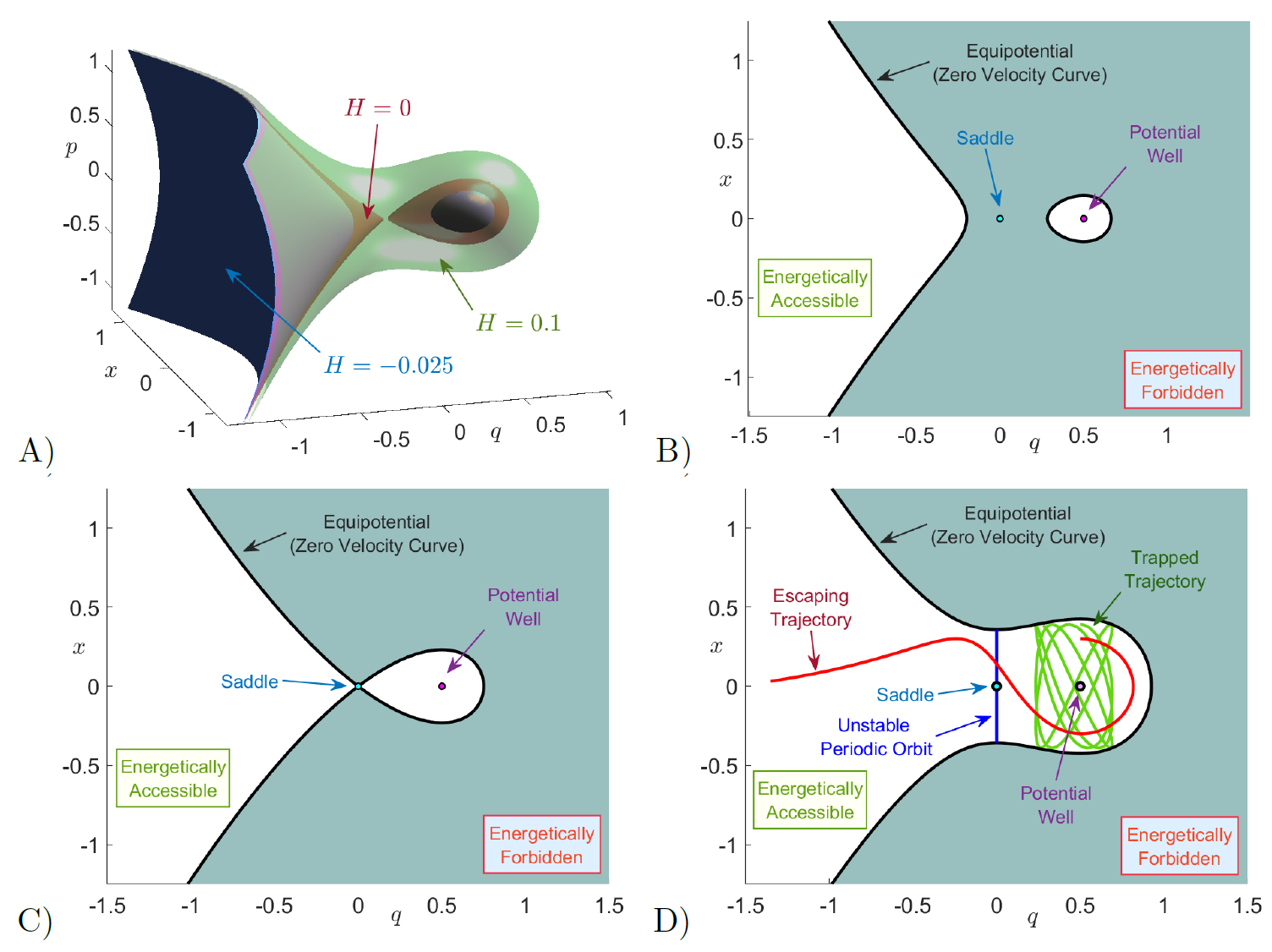
\begin{equation} \begin{split} \mathcal{C}(H_0) &= \left\lbrace (q,x) \in \mathbb{R}^2 \; \big|\; V(q,x) \leqslant H_0 \right\rbrace \\ &= \left\lbrace (q,x) \in \mathbb{R}^2 \; \big|\; - \sqrt{\mu} \, q^2 + \frac{\alpha}{3} \,q^3 + \dfrac{\omega^2}{2} x^2 + \dfrac{\varepsilon}{2} \left(x-q\right)^2 \leqslant H_0 \right\rbrace \end{split} \;, \label{eq:hillsreg} \end{equation}which denotes configurations with positive kinetic energy, and is known in Celestial Mechanics as the Hill's region. The boundary of \mathcal{C}(H_0) is defined as the locus of points in the (q,x) plane where the kinetic energy is zero, that is H_0 = V(q,x), and is called the zero velocity curve. The configuration space coordinates of the trajectories can only evolve inside the Hill's region, shown as white regions in Fig. fig:3. In order to identify the invariant manifolds, we take two dimensional slices of the energy surface and determine the intersection of the invariant manifolds with these low-dimensional slices. In particular, we calculate LDs and compare with qualitative understandings from Poincar\'e surfaces of section (SOSs). The isoenergetic SOSs chosen are:
\begin{align} \mathcal{U}_{qp}^{+} &= \left\lbrace (q,x,p,p_x) \in \mathbb{R}^4 \; \big| \; x = 0 \; ,\; p_x(q,x,p;H_0) \geq 0 \right\rbrace \label{eq:sos_qp} \\[.1cm] \mathcal{U}_{xp_x}^{+} &= \left\lbrace (q,x,p,p_x) \in \mathbb{R}^4 \; \big| \; q = q_e \; , \; p(q,x,p_x;H_0) \geq 0 \right\rbrace \label{eq:sosxpx} \end{align}where q_e is the first configuration space coordinate of the center equilibrium \mathbf{x}_2^e in Eq. \eqref{eq:cfSp_eqCoords}.
We focus first on describing the dynamics for the uncoupled system (\varepsilon = 0). In this case the ''reaction'' and ''bath'' DoF are uncoupled, and therefore, the system is integrable and the trajectories are regular. The total energy can be partitioned among each DoF separately:
\begin{equation} H(q,x,p,p_x) = \underbrace{\frac{1}{2} p^2 - \sqrt{\mu} \, q^2 + \frac{\alpha}{3} q^3}_{H_r(q,p)} + \underbrace{\frac{1}{2} \, p_x^2 + \frac{\omega^2}{2} x^2}_{H_b(x,p_x)} \;, \end{equation}where H_r and H_b are the Hamiltonians for the reaction and bath DoF respectively. Given a fixed total energy of the system H_0, the necessary condition in order for reaction to take place is that the total energy is above that of the barrier of the PES located at the origin, which is zero. For H_0 \leq 0 the energy surface divides phase space into two disconnected regions as illustrated in Fig. fig:3, so that we have bounded motion in the potential well region. In Fig. fig:4, we compare the bounded trajectories (regular dynamics) of the system for H_0 = 0 by computing LDs and Poincar\'e section on the SOS \mathcal{U}_{qp}^{+} in Eq. \eqref{eq:sos_qp}. Both methods clearly recover, the trajectories on tori, as known for integrable Hamiltonian systems [42], that foliate the energy surface. We observe that the high values (white regions in Fig. fig:4 in the LD contour map recover the quasiperiodic trajectories, which is a consequence of the relationship between the convergence of time averages of LDs with the Ergodic Partition Theorem as explained in [40].
When the energy of the system is above the barrier, that is H_0 > 0, the topology of the energy surface changes and a phase space bottleneck opens up in the barrier region allowing the escape from the well as shown in Fig.~fig:3 D). Thus, reaction can take place when trajectories cross the bottleneck, and we can define reaction when the q configuration coordinae changes sign, passing from q > 0 to q < 0 or vice-versa. Therefore, q=0 is a natural choice for defining in phase space a dividing surface (DS) separating reactants (bounded motion in the potential well region) from products (escape to infinity). Hence, the isoenergetic DS is given by:
\begin{equation} \mathcal{D}(H_0) = \left\{ (q,x,p,p_x) \in \mathbb{R}^4 \; | \; q = 0 \;,\; 2H_0 = p^2 + p_x^2 + \omega^2 x^2 \right\} \;, \end{equation}which has the geometry of a 2-sphere, that is S^2 in the three-dimensional energy hypersurface. To be precise, it is an ellipsoid with semi-major axis \sqrt{2H_0} in the p, p_x axis, and \sqrt{2H_0}/\omega in the x axis. This ellipsoid has two hemispheres, known as the forward and backward DS with the form:
\begin{equation} \begin{split} \mathcal{D}_f(H_0) &= \left\{ (q,x,p,p_x) \in \mathbb{R}^4 \; | \; q = 0 \;,\; p =- \sqrt{2H_0 - p_x^2 - \omega^2 x^2} \right\} \\[.1cm] \mathcal{D}_b(H_0) &= \left\{ (q,x,p,p_x) \in \mathbb{R}^4 \; | \; q = 0 \;,\; p = +\sqrt{2H_0 - p_x^2 - \omega^2 x^2} \right\} \end{split} \;. \end{equation}Forward reaction occurs when trajectories cross \mathcal{D}_f and escape from the potential well, and backward reaction when trajectories cross \mathcal{D}_b and enter the well region. The forward and backward DS meet at the equator along the NHIM given by:
\begin{equation} \mathcal{N}(H_0) = \left\{ (q,x,p,p_x) \in \mathbb{R}^4 \; | \; q = p = 0 \;,\; 2H_0 = p_x^2 + \omega^2 x^2 \right\} \;, \end{equation}which has the topology of S^1. To be precise, it is an ellipse with semiaxis \sqrt{2H_0} in the p_x direction and \sqrt{2H_0}/\omega in the x direction. As discussed earlier, for a 2 DoF Hamiltonian the NHIM is an unstable periodic orbit which extends the influence of the index-1 saddle equilibrium point of the PES, a configuration space concept, into phase space. We note that for H_0 > 0 the NHIM is the correct phase space structure that anchors the barriers to the reaction and carries the effect of the index-1 saddle equilibrium point to a range of energies as given by Moser's generalization of Lyapunov Subcenter Manifold Theorem [34]. The stable and unstable manifolds of the UPO are:
\begin{equation} \mathcal{W}^s = \Gamma \cup \mathcal{W}^s_l \quad , \quad \mathcal{W}^u = \Gamma \cup \mathcal{W}^u_l \;, \end{equation}where \Gamma is the homoclinic orbit:
\begin{equation} \Gamma = \left\{ (q,x,p,p_x) \in \mathbb{R}^4 \; | \; q > 0 \;,\; H_r(q,p) = 0 \;,\; H_b(x,p_x) = H_0 \right\} \;, \end{equation}and the left branches are:
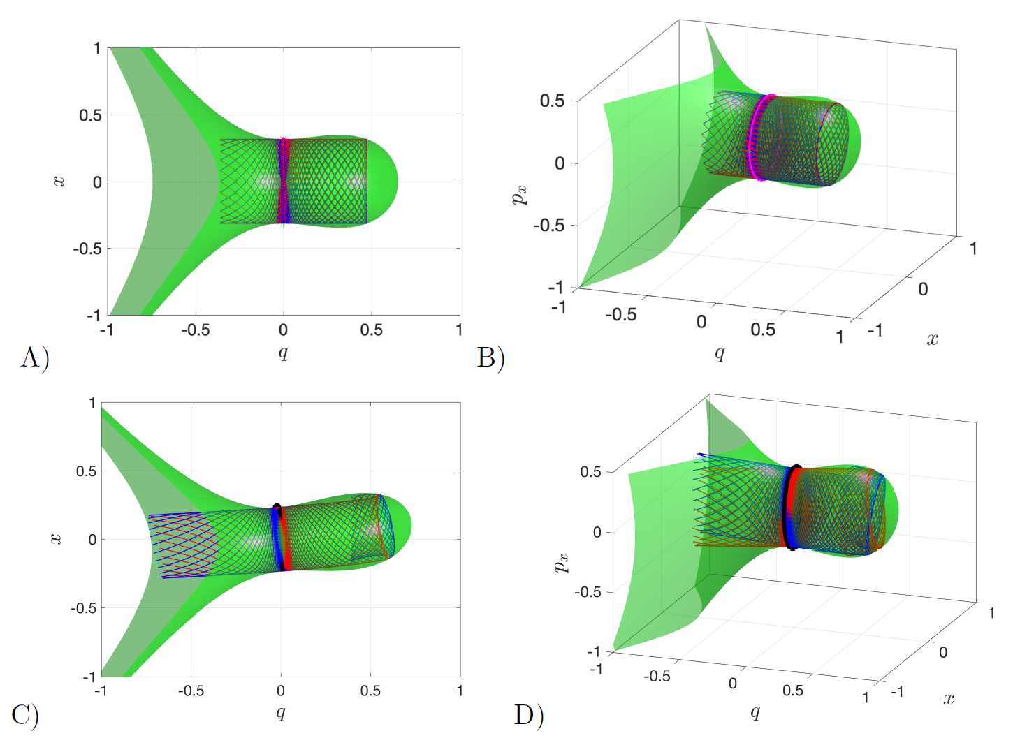
\begin{equation} \begin{split} \mathcal{W}^s_l &= \left\{ (q,x,p,p_x) \in \mathbb{R}^4 \; | \; q < 0 \:,\; p > 0 \;,\; H_r(q,p) = 0 \;,\; H_b(x,p_x) = H_0 \right\} \\[.2cm] \mathcal{W}^u_l &= \left\{ (q,x,p,p_x) \in \mathbb{R}^4 \; | \; q < 0 \:,\; p < 0 \;,\; H_r(q,p) = 0 \;,\; H_b(x,p_x) = H_0 \right\} \end{split} \;. \end{equation}Notice that the stable and unstable manifolds have the structure of a cartesian product of a curve in the (q,p) saddle space and an ellipse in the (x,p_x) center space, and thus become cylindrical (or tube) manifolds. We show the energy surface for the uncoupled case (\varepsilon = 0) in Fig. fig:3 A) for three energy values, where the bottleneck only opens for H_0 > 0. The NHIM computed using differential correction and continuation, and its invariant manifolds computed using globalization are shown in Fig. fig:5A) for H_0 = 0.05 and \varepsilon = 0.
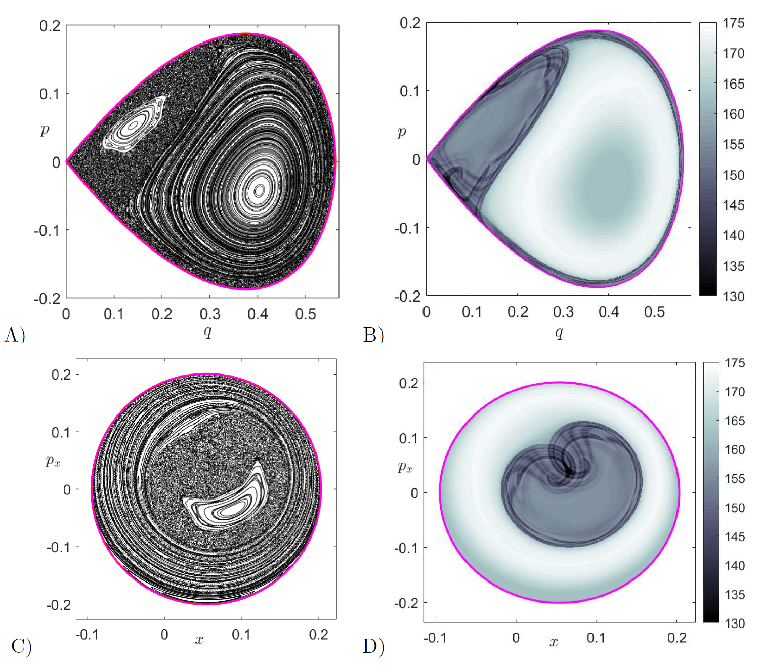
We discuss next the dynamics of the system when the reactive and bath DoF are coupled, i.e. \varepsilon \neq 0, and we do so for \varepsilon small. We can thus think about the resulting dynamics as a perturbation of the uncoupled case. Given an energy of the system below that of the barrier, that is H_0 \leq 0, the phase space bottleneck is closed and trajectories are trapped in the potential well region. However, due to the perturbation, the regular motion that existed on the tori in the uncoupled system is destroyed as given by the KAM theorem, and therefore chaotic motion arises in some regions of the phase space. We illustrate the system's behavior for the energy H_0 = 0 (energy of the index-1 saddle) in Fig. fig:6 using LDs and Poincar\'e maps on the SOSs described in Eqs. \eqref{eq:sos_qp} and \eqref{eq:sosxpx}. We observe that there is a distinct correlation between the qualitative dynamics revealed by the Lagrangian descriptor (LD) contour maps and Poincar\'e sections. That is, chaotic regions of phase space which appear as a sea of points in the Poincar\'e section and hide the underlying structures of stable and unstable manifolds are completely resolved by LD contour maps where the tangled geometry of the manifolds is revealed by the points where the function is non-differentiable and attains a local minimum as has been shown in [40], [38], [17]. The capability of LDs to identify the phase space structures relevant in chemical reaction dynamics can also be found in recent literature [43], [44], [45], [24]. In addition, the generation of Poincar\'e sections relies on tracking the crossing of a 2D surface which can not be guaranteed in high dimensional phase space, while LDs just accumulate a positive scalar quantity along the trajectory and thus have potential to reveal high dimensional phase space structures.
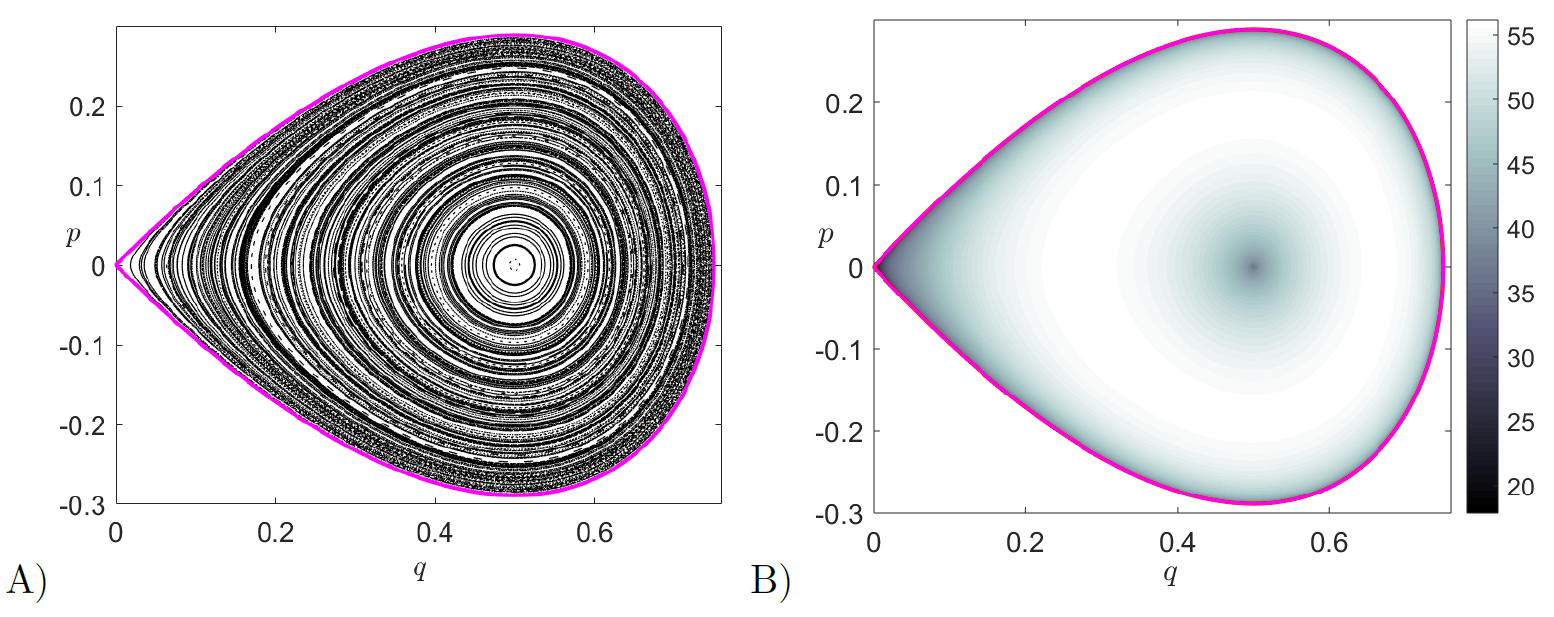
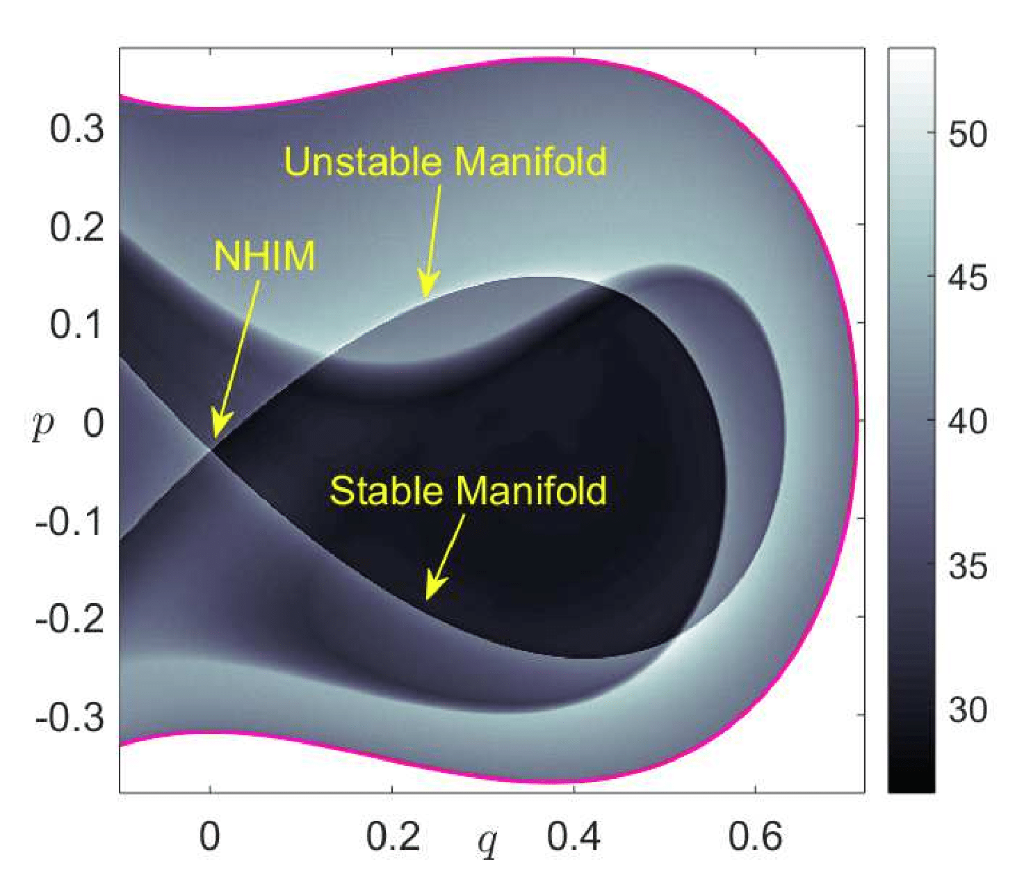
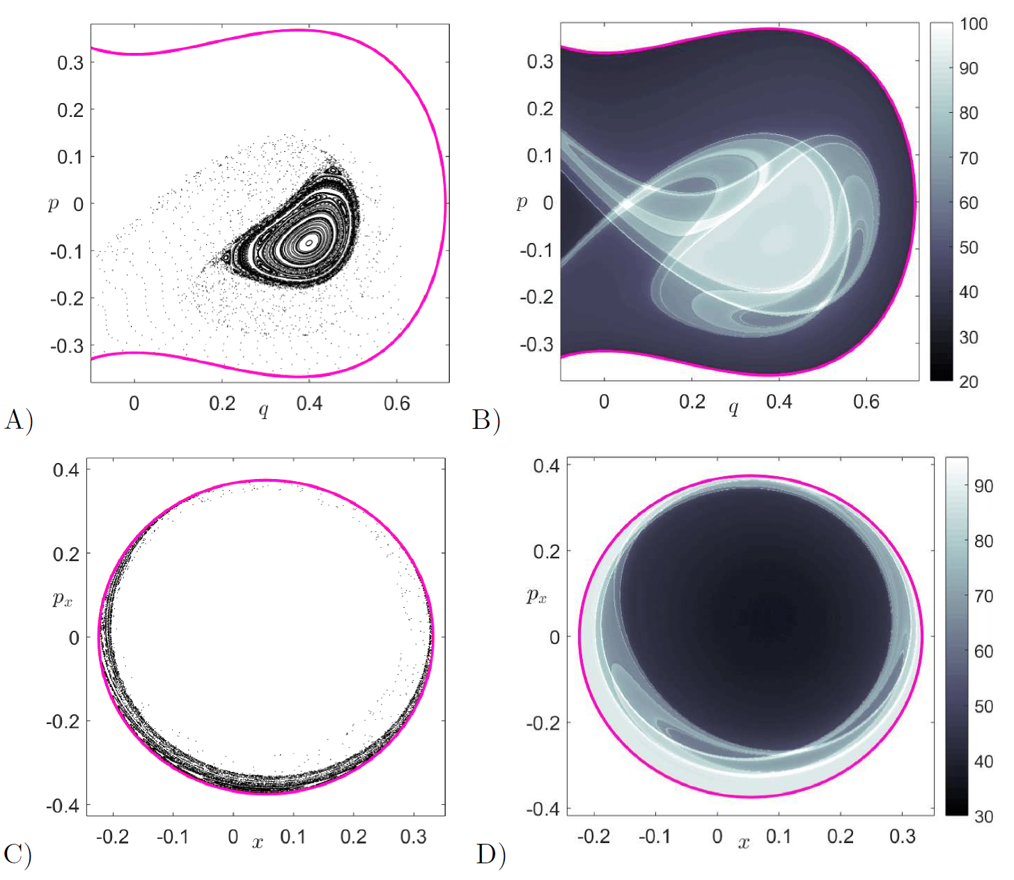
To finish the analysis, we consider the dynamics when the total energy is above that of the index-1 saddle, that is H_0 > 0, and in particular we will set H_0 = 0.05 in our computations. In this situation, a phase space bottleneck opens up in the barrier region, as shown in Fig. fig:3. In order to describe the structures that mediate reaction dynamics, that is the NHIM (or unstable periodic orbit) and its stable and unstable manifolds, we use differential correction and continuation along with globalization as described in [36], [37], [38], [17]. In Fig. fig:5 panels C) and D), we show the cylindrical manifolds along with the energy surface and the unstable periodic orbit. In order to recover the homoclinic tangle geometry of the invariant manifolds, we calculate LDs on the surfaces of section \mathcal{U}^{+}_{qp} and \mathcal{U}^{+}_{xp_x}, and compare with the direct numerical construction of these invariant manifolds. This LD based diagnostic is similar to performing a ''phase space tomography'' of the high dimensional phase space structures using a low dimensional slice. In Fig. fig:7 we show the computation of variable time LDs for an integration time \tau = 10 on the slice \mathcal{U}^{+}_{qp}. We observe that Lagrangian descriptors clearly identify the location of the stable and unstable manifolds and the NHIM at the intersection of the invariant manifolds. Since we are using a small integration time of \tau = 10 to compute LDs, the complete geometry of the homoclinic tangle is not fully revealed. Therefore, in order to recover a more complete and intricate dynamical picture of the homoclinic tangle, the integration time to compute LDs has to be increased. This is shown in Fig. fig:8B), where \tau = 30 and we observe that the regular motion obtained in the middle of the Poincar\'e section displayed in Fig. fig:8 A) corresponds to trajectories that remain trapped in the potential well region and never escape. The trapped dynamics on the tori are also captured by the LD contour map shown in Fig. fig:8B) which also reveals the homoclinic tangle of the stable and unstable manifolds and the resulting lobe dynamics [46]. We note that in all these computations we are using the variable time definition of LDs, since the open potential surface causes trajectories to escape to infinity through the bottleneck in finite time, resulting in NaN values in the LD contour map and would hide the important underlying phase space structures making the interpretation of results difficult. In addition, when we analyze the dynamics using Poincar\'e sections, we cannot ensure that trajectories return to the surface of section when the dynamical behavior of escaping to infinity is possible in the system. This will result in blank regions in the Poincar\'e sections as shown in Fig. fig:8A) and C). However, we note that trapped trajectories in the potential well corresponding to regular (motion on the tori) and chaotic motion are highlighted as expected in the Poincar\'e sections. These trajectories are non-reactive and will remain so until they satisfy the sufficient condition for reaction which is entering the cylindrical manifolds.
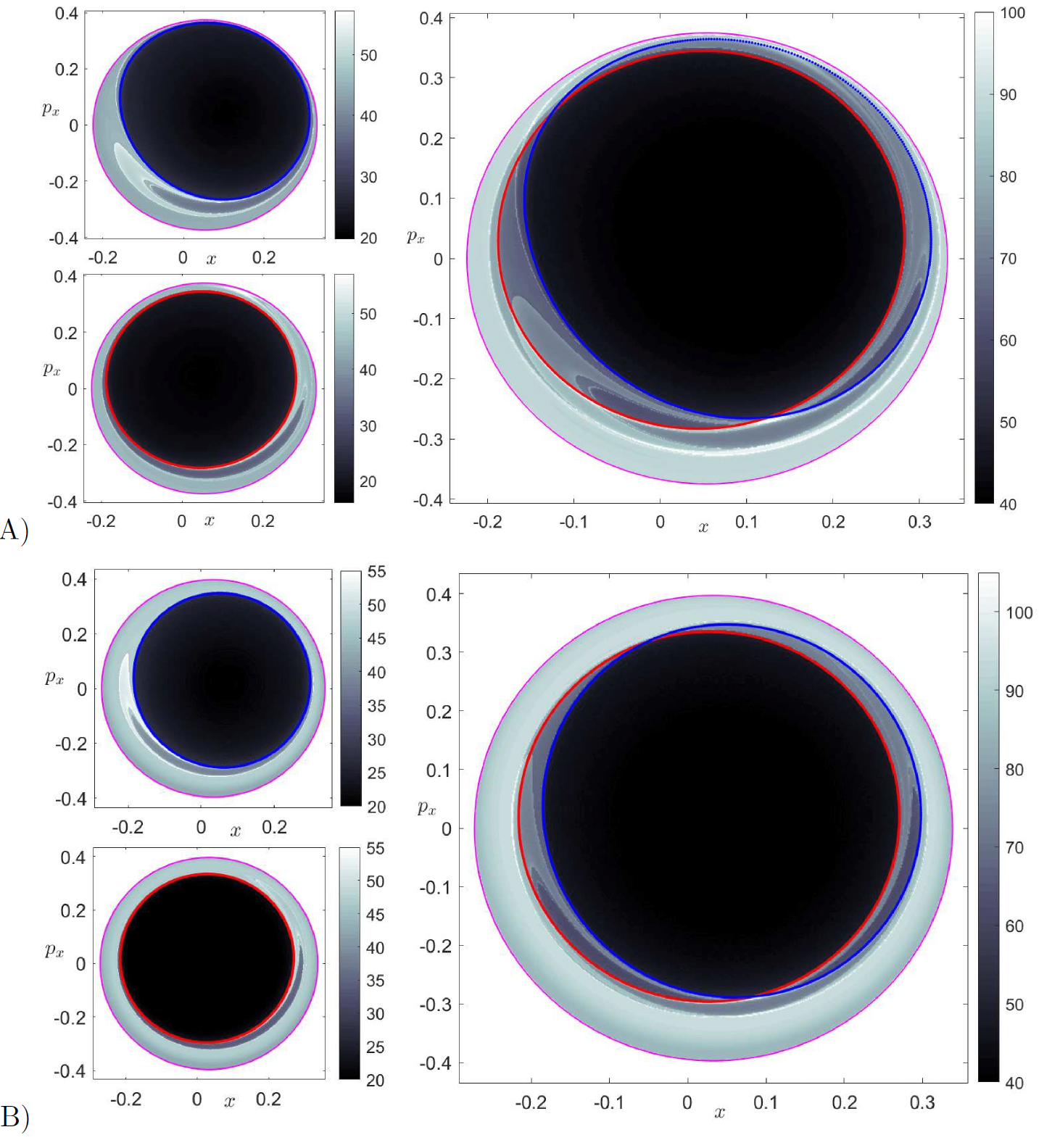
Identifying the regions inside the cylindrical (tube) stable and unstable manifolds can be done using globalization or using the LD contour map on appropriate isoenergetic surfaces. We compute LD contour maps to recover the intersections of these tube manifolds with the surface of section in Eq. \eqref{eq:sosxpx}. The intersection of the invariant manifolds with the isoenergetic surface of section yields topological ellipses, known in the chemical reactions literature as reactive islands [47], [48], [49], [50] which are of paramount importance for the computation of reaction rates/fraction. In order to illustrate the capability of LDs to recover the reactive island structure, we have compared the LD contour map and manifold intersection with the surface of section \mathcal{U}^{+}_{xp_x} obtained using globalization in Fig. fig:9. We have shown the first intersection of the stable and unstable manifolds with the surface of section as a blue/red curve superimposed on the LD contour map. We observe that the points at which the LDs scalar field is non-differentiable and the manifolds intersections are in agreement, thus verifying the LD based identification of reactive islands. We also observe that successive folds and resulting intersections of the tube manifolds with the surface of section are also revealed by LDs. We note here that the first intersection of the manifolds encloses a large phase space volume in the potential well which indicates that a large portion of the potential well escapes to infinity through the bottleneck. This is despite the fact that we have chosen a very small value for the energy of the system, H_0 = 0.05, compared to the energy of the barrier. This is a consequence of using a high coupling strength, \varepsilon = 0.25, which makes the vase-like shaped potential well region small and narrow, since the center equilibrium point at the bottom of the potential well approaches the index-1 saddle equilibrium point at the origin as \varepsilon is increased. Movies illustrating the change in both the shape of the energy surface and the equipotentials in configurations space as we vary the coupling strength can be found at the links https://youtu.be/kYklCrSwtls and https://youtu.be/0FNChWVM6nU respectively. We can see that the effect of increasing the coupling strength from zero is to tilt and squeeze the vase-like shape of the energy surface that qualitatively increases the number of reactive trajectories. This action of tilting and squeezing of the vase-like container (boundary defined by the total energy surface) is to pour out its contents (the reactive trajectories) and hence the increase in reaction fraction. A quantitative investigation of this phenomenon is current work in progress and beyond the scope of this chapter.
References
- T. Komatsuzaki and R. S. Berry, “Local regularity and non-recrossing path in transition state: a new strategy in chemical reaction theories,” J. Mol. Struct. THEOCHEM, vol. 506, pp. 55–70, 2000.
- T. Uzer, C. Jaffé, J. Palacián, P. Yanguas, and S. Wiggins, “The geometry of reaction dynamics,” Nonlinearity, vol. 15, no. 4, p. 957, 2002.
- T. Komatsuzaki and R. S. Berry, “A dynamical propensity rule for transitions in chemical reactions,” J. Phys. Chem. A, vol. 106, pp. 10945–10950, 2002.
- R. S. MacKay, “Flux over a saddle,” Phys. Lett. A, vol. 145, pp. 425–427, 1990.
- H. Waalkens and S. Wiggins, “Direct construction of a dividing surface of minimal flux for multi-degree-of-freedom systems that cannot be recrossed,” J. Phys. A: Math. Gen., vol. 37, no. 35, p. L435, 2004.
- E. P. Wigner, “The transition state method,” Trans. Faraday Soc., vol. 34, pp. 29–40, 1938.
- E. P. Wigner, “Some remarks on the theory of reaction rates,” J. Chem. Phys., vol. 7, pp. 646–650, 1939.
- H. Waalkens, R. Schubert, and S. Wiggins, “Wigner’s dynamical transition state theory in phase space: classical and quantum,” Nonlinearity, vol. 21, pp. R1–R118, 2008.
- S. Wiggins, Global bifurcations and chaos: Analytical methods. Springer-Verlag, 1988.
- S. Wiggins, “On the geometry of transport in phase space I. Transport in k degree-of-freedom Hamiltonian systems, 2 \le k < ∞,” Physica D, vol. 44, pp. 471–501, 1990.
- S. Wiggins, Normally hyperbolic invariant manifolds in dynamical systems, vol. 105. Springer Science & Business Media, 2013.
- P. Pechukas and F. J. McLafferty, “On transition state theory and the classical mechanics of collinear collisions,” J. Chem. Phys., vol. 58, no. 4, pp. 1622–1625, 1973.
- P. Pechukas and E. Pollak, “Trapped trajectories at the boundary of reactivity bands in molecular collisions,” J. Chem. Phys., vol. 67, no. 12, pp. 5976–5977, 1977.
- E. Pollak and P. Pechukas, “Transition states, trapped trajectories, and bound states embedded in the continuum,” J. Chem. Phys., vol. 69, pp. 1218–1226, 1978.
- P. Pechukas and E. Pollak, “Classical transition state theory is exact if the transition state is unique,” J. Chem. Phys., vol. 71, no. 5, pp. 2062–2068, 1979.
- S. Wiggins, L. Wiesenfeld, C. Jaffé, and T. Uzer, “Impenetrable barriers in phase-space,” Physical Review Letters, vol. 86, no. 24, pp. 5478–5481, 2001.
- V. J. García-Garrido, S. Naik, and S. Wiggins, “Tilting and Squeezing: Phase space geometry of Hamiltonian saddle-node bifurcation and its influence on chemical reaction dynamics,” arXiv preprint:1907.03322 (Accepted in International Journal of Bifurcation and Chaos)., 2019.
- D. Hathcock and J. P. Sethna, “Renormalization Group for Barrier Escape: Crossover to Intermittency,” arXiv preprint:1902.07382, 2019.
- J. Husson, M. Dogterom, and F. Pincet, “Force spectroscopy of a single artificial biomolecule bond: The Kramers’ high-barrier limit holds close to the critical force,” The Journal of Chemical Physics, vol. 130, no. 5, p. 051103, Feb. 2009.
- N. J. Miller and S. W. Shaw, “Escape statistics for parameter sweeps through bifurcations,” Physical Review E, vol. 85, no. 4, p. 046202, Apr. 2012.
- C. Herbert and F. Bouchet, “Predictability of escape for a stochastic saddle-node bifurcation: When rare events are typical,” Physical Review E, vol. 96, no. 3, p. 030201, Sep. 2017.
- F. Borondo, A. A. Zembekov, and R. M. Benito, “Quantum manifestations of saddle-node bifurcations,” Chemical Physics Letters, vol. 246, no. 4, pp. 421–426, 1995.
- F. Borondo, A. A. Zembekov, and R. M. Benito, “Saddle-node bifurcations in the LiNC/LiCN molecular system: Classical aspects and quantum manifestations,” The Journal of chemical physics, vol. 105, no. 12, pp. 5068–5081, 1996.
- F. Revuelta, R. M. Benito, and F. Borondo, “Unveiling the chaotic structure in phase space of molecular systems using Lagrangian descriptors,” Physical Review E, vol. 99, no. 3, p. 032221, 2019.
- N. De Leon and B. J. Berne, “Intramolecular rate process: Isomerization dynamics and the transition to chaos,” The Journal of Chemical Physics, vol. 75, no. 7, pp. 3495–3510, Oct. 1981.
- K. A. Mitchell, J. P. Handley, B. Tighe, J. B. Delos, and S. K. Knudson, “Geometry and topology of escape. I. Epistrophes,” Chaos: An Interdisciplinary Journal of Nonlinear Science, vol. 13, no. 3, pp. 880–891, Sep. 2003.
- K. A. Mitchell, J. P. Handley, J. B. Delos, and S. K. Knudson, “Geometry and topology of escape. II. Homotopic lobe dynamics,” Chaos: An Interdisciplinary Journal of Nonlinear Science, vol. 13, no. 3, pp. 892–902, Sep. 2003.
- K. A. Mitchell, J. P. Handley, B. Tighe, A. Flower, and J. B. Delos, “Chaos-Induced Pulse Trains in the Ionization of Hydrogen,” Physical Review Letters, vol. 92, no. 7, Feb. 2004.
- K. A. Mitchell, J. P. Handley, B. Tighe, A. Flower, and J. B. Delos, “Analysis of chaos-induced pulse trains in the ionization of hydrogen,” Physical Review A, vol. 70, no. 4, Oct. 2004.
- K. A. Mitchell and J. B. Delos, “The structure of ionizing electron trajectories for hydrogen in parallel fields,” Physica D: Nonlinear Phenomena, vol. 229, no. 1, pp. 9–21, May 2007.
- K. A. Mitchell and B. Ilan, “Nonlinear enhancement of the fractal structure in the escape dynamics of Bose-Einstein condensates,” Physical Review A, vol. 80, no. 4, Oct. 2009.
- L. Wang, H. F. Yang, X. J. Liu, H. P. Liu, M. S. Zhan, and J. B. Delos, “Photoionization microscopy of the hydrogen atom in parallel electric and magnetic fields,” Physical Review A, vol. 82, no. 2, Aug. 2010.
- M. Spivak, A Comprehensive Introduction to Differential Geometry. Publish or Perish, Incorporated, 1999.
- S. Wiggins, Introduction to Applied Nonlinear Dynamical Systems and Chaos, vol. 2. Springer Science & Business Media, 2003.
- S. Wiggins, L. Wiesenfeld, C. Jaffé, and T. Uzer, “Impenetrable Barriers in Phase-Space,” Physical Review Letters, vol. 86, no. 24, pp. 5478–5481, 2001.
- W. S. Koon, M. W. Lo, J. E. Marsden, and S. D. Ross, Dynamical systems, the three-body problem and space mission design. Marsden books, 2011, p. 327.
- S. Naik and S. D. Ross, “Geometry of escaping dynamics in nonlinear ship motion,” Communications in Nonlinear Science and Numerical Simulation, vol. 47, pp. 48–70, Jun. 2017.
- S. Naik and S. Wiggins, “Finding normally hyperbolic invariant manifolds in two and three degrees of freedom with Hénon-Heiles type potential,” Phys. Rev. E, vol. 100, no. 2, p. 022204, 2019.
- A. M. Mancho, S. Wiggins, J. Curbelo, and C. Mendoza, “Lagrangian descriptors: A method for revealing phase space structures of general time dependent dynamical systems,” Communications in Nonlinear Science and Numerical Simulation, vol. 18, no. 12, pp. 3530–3557, 2013.
- C. Lopesino, F. Balibrea-Iniesta, V. J. García-Garrido, S. Wiggins, and A. M. Mancho, “A Theoretical Framework for Lagrangian Descriptors,” International Journal of Bifurcation and Chaos, vol. 27, no. 01, p. 1730001, 2017.
- A. Junginger, L. Duvenbeck, M. Feldmaier, J. Main, G. Wunner, and R. Hernandez, “Chemical dynamics between wells across a time-dependent barrier: Self-similarity in the Lagrangian descriptor and reactive basins,” The Journal of chemical physics, vol. 147, no. 6, p. 064101, 2017.
- K. R. Meyer, G. R. Hall, and D. Offin, Introduction to Hamiltonian Dynamical Systems and the N-Body Problem. Springer, 2009.
- G. T. Craven and R. Hernandez, “Deconstructing field-induced ketene isomerization through Lagrangian descriptors,” Physical Chemistry Chemical Physics, vol. 18, no. 5, pp. 4008–4018, 2016.
- A. S. Demian and S. Wiggins, “Detection of Periodic Orbits in Hamiltonian Systems Using Lagrangian Descriptors,” International Journal of Bifurcation and Chaos, vol. 27, no. 14, p. 1750225, 2017.
- S. Naik, V. J. García-Garrido, and S. Wiggins, “Finding NHIM: Identifying high dimensional phase space structures in reaction dynamics using Lagrangian descriptors,” Communications in Nonlinear Science and Numerical Simulation, vol. 79, p. 104907, 2019.
- D. Beigie and S. Wiggins, “Dynamics associated with a quasiperiodically forced Morse oscillator: Application to molecular dissociation,” Physical Review A, vol. 45, no. 7, pp. 4803–4827, 1992.
- N. De Leon, M. A. Mehta, and R. Q. Topper, “Cylindrical manifolds in phase space as mediators of chemical reaction dynamics and kinetics. I. Theory,” The Journal of Chemical Physics, vol. 94, no. 12, pp. 8310–8328, 1991.
- N. De Leon, M. A. Mehta, and R. Q. Topper, “Cylindrical manifolds in phase space as mediators of chemical reaction dynamics and kinetics. II. Numerical considerations and applications to models with two degrees of freedom,” The Journal of Chemical Physics, vol. 94, no. 12, pp. 8329–8341, 1991.
- N. De Leon, “Cylindrical manifolds and reactive island kinetic theory in the time domain,” The Journal of Chemical Physics, vol. 96, no. 1, pp. 285–297, 1992.
- S. Patra and S. Keshavamurthy, “Detecting reactive islands using Lagrangian descriptors and the relevance to transition path sampling,” Physical Chemistry Chemical Physics, vol. 20, no. 7, pp. 4970–4981, 2018.